The Stack Below the Stack, a 3-part series on how modern LLM inference actually works, told through a single DeepSeek V4 dtype bug.
- Part 1 · Physics of a request : why the first token is a different problem from every token after it, and why batching exists.
- Part 2 · Below Python : what actually runs under
vllm serve, and why the escape hatches failed.- Part 3 (this post) · Serving at scale: recipes, fleets, traffic shapes, and the bug resolved layer by layer.
Catch-up:
- Part 1 was the physics of one request (prefill vs decode, the roofline, the batch crossover $B^{\star}$).
- Part 2
was the machinery under
vllm serve(the GPU, kernels, and compilers) and why the opening bug lived in a fused C++ op that--enforce-eagercould not reach. - Part 3: this part composes both into how a recipe like DeepSeek’s
DP+EP+ FP8 KV + chunked prefill is built from those pieces: fleets, disaggregation, speculation, agents, reasoning effort, and it closes by re-reading the DeepSeek V4 dtype bug with every layer named.
The catch is that “serving at scale” is not one thing: it is a dozen distinct techniques, each with its own advantage and trade-off. If one reads those different techniques end-to-end they can feel like a grab bag: PagedAttention, then quantization, then LoRA, then disaggregation, then reasoning effort. So before the details, let us understand the shape of the whole thing.
Every technique here is a lego block, and each block does exactly one of three jobs: it moves fewer bytes per token, it launches fewer or cheaper kernels, or it decides which pool runs which phase of the request. Figure 1 snaps those blocks into the tiers they actually occupy, from the traffic that drives demand down to the silicon that answers it.

The colors say which latency lever each block moves: green blocks buy back TTFT (the prefill side), blue blocks buy back TPOT (the decode side), and amber blocks free up KV capacity. Grey blocks do not move a single latency number: the traffic that sets the workload, the control plane and substrate that hold everything up, and multi-LoRA, which stretches capacity across variants. The table below is the reading order for the rest of this part, one row per stretch of sections, with the map tier each one lives on:
| Sections | What they cover | Tier on the map |
|---|---|---|
| 1 | Serving engine: batching, PagedAttention, parallelism, chunked prefill, prefix caching | Per-replica engine |
| 2-4 | Quantization, multi-LoRA, speculative decoding | Byte/token economy |
| 5 | Disaggregating prefill and decode | Fleet topology |
| 6 | Outside CUDA: other accelerators | Substrate |
| 7 | Scheduling, queueing, fleet routing | Fleet control plane |
| 8-9 | Agentic and reasoning-effort traffic | Traffic shape |
| 10-11 | The bug re-read, and the takeaways | Wrap-up |
One number is worth holding onto before we get into the sections: what does all of this actually buy once we stack it? Start with a trillion-parameter model on a stock engine, nothing applied, and a request sits somewhere ~30-40 tps. Now add the different lego blocks one at a time:
- Quantizing to 4-bit is roughly 2× (we stream about a quarter of the bytes, minus the dequant tax).
- A decode speculator matched to our traffic (a draft model or built-in MTP head) is another 2×.
- Splitting prefill and decode across separate pools, once we have the hardware and the traffic to keep both busy, is another 2×.
- A newer runtime with current kernels adds a double-digit percentage on top of that.
Because these attack different bottlenecks, they compose multiplicatively, so three honest 2×s already put us near 8×, and the industry target for a heavily optimized deployment is on the order of 10× over the naive baseline. That is the shape of the payoff, and it is why serving is its own discipline: the gains here are measured in multiples. The rest of this part is where each of those multipliers comes from.
1. The serving engine layer: vLLM and its peers
The serving engine is where all those layers finally meet the request path: the scheduler, the KV cache manager, the OpenAI-compatible API. It gets the most attention in this part for a simple reason: nearly every request spends nearly all of its life inside it, so this is where most of the levers live. It is also where the DeepSeek bug surfaced (profile_run, the parallelism flags, the fused MoE router), even though the contract that actually broke lived a layer down.
vLLM is the application server of this stack: a checkpoint goes in, it manages the GPU memory and the schedule, runs the forward passes, and streams tokens back out over HTTP. It began as a 2023 paper (“Efficient Memory Management for Large Language Model Serving with PagedAttention”) and is now the de facto open-source default.
1.1 Choosing an engine: the popular options
I use vLLM as the worked example throughout this part because that is where the DeepSeek bug lived, but it is not the only serving engine, and for some workloads it is not the obvious first choice. Three engines dominate open and semi-open production serving today, and a few more show up often enough that we will meet them in the wild:
| Engine | Origin and bet | Strengths | Reach for it when |
|---|---|---|---|
| vLLM | PagedAttention (Berkeley, SOSP 2023); the broadest community | Widest model and hardware coverage, usually day-zero support for new architectures, OpenAI-compatible API | You want the safe default, the newest models on release day, or the largest ecosystem |
| SGLang | RadixAttention plus a frontend DSL for programming LLM calls | First-class prefix reuse across requests, fast structured and constrained output (JSON, grammars), a strong MoE and DeepSeek production track record | Traffic has heavy shared prefixes or is agentic, you need structured output, or you serve DeepSeek-class MoE models at scale |
| TensorRT-LLM | NVIDIA, ahead-of-time compiled engines | Highest peak throughput on NVIDIA silicon, tight kernel and quantization integration | You are NVIDIA-only, latency-critical, and can afford an AOT build and tuning step per model |
| Hugging Face TGI | Hugging Face Text Generation Inference | Tight HF Hub / Transformers integration, familiar ops story for teams already on the Hub | You want the Hub-native path more than peak tokens/s |
| LMDeploy | InternLM / SenseTime | Strong TurboMind backend, solid quantization story, popular in China-facing deployments | You are already in that ecosystem or need its TurboMind kernels |
| llama.cpp / Ollama | Georgi Gerganov et al.; Ollama as the ergonomic wrapper | Runs well on CPU and consumer GPUs, tiny ops surface, great for local and edge | Laptops, air-gapped boxes, or “just make it run” demos rather than multi-node fleets |
The differences among the first three are smaller than the online debates suggest. All three implement continuous batching, a paged KV cache, chunked prefill, and the parallelism strategies below; the RadixAttention and PagedAttention ideas have largely converged, and vLLM’s Automatic Prefix Caching is its answer to RadixAttention (covered below under prefix caching). TGI and LMDeploy speak the same vocabulary with different defaults. llama.cpp and Ollama sit in a different product niche: they are not trying to win the multi-node goodput race in the first place.
The practical decision usually comes down to a few questions: does our target model have day-zero support, does our traffic have enough shared prefix to reward SGLang’s radix tree, are we locked to NVIDIA hardware, and are we serving a fleet or a laptop? For DeepSeek V4 specifically, both vLLM and SGLang are first-class choices; I reached for vLLM here only because that’s where I hit the bug where I already had vLLM setup.
As a result, even though the rest of this section uses vLLM to make the serving layer concrete, the concepts (PagedAttention, the parallelism strategies, chunked prefill, and prefix caching) map onto SGLang and TensorRT-LLM with different names and knobs.
1.2 PagedAttention
The KV cache (the running memory of attention keys and values for each in-flight conversation, explained in the KV cache post ) was historically the biggest source of GPU memory waste. Three things ate the memory: each request reserved space for its worst-case sequence length, beam search duplicated the shared prefix across beams, and variable-length sequences left the rest fragmented.
PagedAttention (Kwon et al., SOSP 2023) borrows directly from OS virtual memory: the KV cache is divided into fixed-size blocks (pages) mapped through a per-request block table. Non-contiguous physical blocks can form a logically contiguous KV sequence, exactly as virtual address spaces do. The result was 2-4× higher throughput than prior systems, almost entirely from packing more concurrent requests into the same GPU memory.
PagedAttention is a buffer pool, the same idea as Postgres shared buffers: fixed-size pages handed out on demand, rather than a private worst-case slab reserved per request. Figure 2 shows the block-table view:
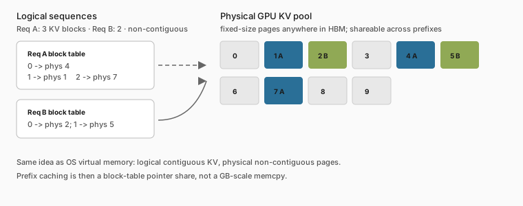
Read the image left to right. On the left, each in-flight request has its own block table, a little lookup that says where its logical KV blocks actually live: Req A’s block 0 sits at physical page 4, its block 1 at page 1, its block 2 at page 7. On the right is the single physical KV pool, one row of fixed-size pages in HBM. The colored pages are the ones currently owned by a request (blue for A, green for B); the grey pages are free. The point the figure is making is that a request’s blocks are scattered across the pool with free pages in between, yet the block table stitches them back into a logically contiguous sequence, so no request ever has to reserve a big contiguous worst-case slab up front.
This is what makes prefix caching cheap, and what lets continuous batching admit more concurrent work without reserving worst-case KV up front.
1.3 Four kinds of parallelism
When the model does not fit on one GPU, we split the work. The four common splits are tensor, pipeline, data, and (for MoE) expert parallelism; they differ in what they shard and which fabric they stress. Figure 3 lays all four side by side, and the bullets under it walk through each in turn.
Two collective operations recur across them, and the distinction matters: an all-reduce sums a tensor across every GPU and hands each one the total (chatty, and it fires once per layer), whereas an all-to-all has every GPU send a different slice to every other (which is how each token’s data reaches wherever its expert happens to live). The DeepSeek V4-Pro H200 recipe is a DP+EP bet, not a TP bet, and that choice is also why the fused router path existed for the opening bug.

Tensor Parallelism (TP) slices each weight matrix across GPUs, so GPU 0 gets columns 1 through 1000 and GPU 1 gets columns 1001 through 2000. Every layer requires all GPUs to synchronize via an all-reduce, so the communication traffic is heavy. It only works well within a node over NVLink; InfiniBand is too slow for this traffic pattern.
Pipeline Parallelism (PP) splits by layers, so Node 1 handles layers 1 through 30 and Node 2 handles layers 31 through 60. Communication is small (just the activations at layer boundaries) and happens only at transitions, so it works well across nodes.
Data Parallelism (DP) runs complete model copies and splits requests between them. No coordination is required for inference, but the model must fit in each GPU group.
Expert Parallelism (EP), specific to MoE models, places different experts on different GPUs. Each token is routed to its selected experts, potentially on different GPUs, via an all-to-all communication step.
In practice we rarely run one of these in isolation; we stack them, and the notation just names which split runs at which level. TP=8 + PP=2 means each of two nodes runs tensor parallelism across its own 8 GPUs, and the two nodes are chained as a two-stage pipeline. DP=16 + EP means 16 data-parallel ranks with one copy of the experts sharded across all of them via DeepEP. Reading one of these strings is just asking, for each split: across how many GPUs, and at what level?
Here is the one idea that makes the DeepSeek recipe click, and it is worth slowing down for. A MoE model is not one uniform block of weights. It has two parts of very different size, and the good layouts parallelize each one differently. The attention weights are small; the expert weights are the overwhelming bulk of the model. So the move is to replicate the small part and shard the big part, in the same deployment.
That is exactly what DP+EP is, and it is why it isn’t the plain data parallelism from the list above. In textbook DP, every rank holds a full copy of the entire model. Under DP+EP, every rank holds a full copy of the small attention weights, but the large expert weights are split across all 16 ranks, so no single rank holds the whole model. vLLM still calls it data-parallel because requests are routed that way, one rank owns a request’s attention from start to finish, but the experts underneath are expert-parallel. It is 16 ranks cooperating on one sharded model, not 16 independent replicas.
Framed that way, the failure of plain TP falls out. For a dense model, where there is only one kind of weight, TP is still the workhorse. For DeepSeek V3 and V4 its efficiency degrades sharply once expert parallelism is on the table, and the two-kinds-of-weights picture is the reason: attention and experts don’t want the same split. Forcing both through TP pays the heavy per-layer all-reduce on every layer, even though the expert compute is sparsely activated and would rather travel as a routed all-to-all.
The vLLM recipe for V4-Pro on H200
recommends DP + EP per node (--data-parallel-size 8 on 8×H200, scaled across nodes for multi-node), using DeepSeek’s open-source DeepEP library for low-latency all-to-all over InfiniBand.
Figure 4 shows that layout on two nodes: attention replicated on every rank, the experts sharded across all of them, and DeepEP carrying the all-to-all within each node and over InfiniBand between them.

Here is how to read that layout, and why it is shaped this way. There are 16 data-parallel ranks in total, one H200 each, eight per node. Two things happen on every rank at once, and they are split along different axes.
- One as we touched on earlier, the attention weights are comparatively small, so every rank keeps a full copy; attention for a request runs entirely on whichever rank that request landed on, with no cross-GPU traffic.
- Two, on the other hand, the expert weights are the bulk of a 1.6T MoE model and are far too large to replicate, so they are sharded: each rank physically holds only a slice of the experts.
That split is what forces the all-to-all. At each MoE layer the router picks, per token, a small set of experts (DeepSeek activates a handful out of hundreds), and those experts can live on any of the 16 ranks.
DeepEP’s all-to-all is the shuffle that makes this work: it ships each token to the rank or ranks that hold its chosen experts, runs the expert FFN there, and ships the results back to be combined. Hops between the eight GPUs inside a node use NVLink; hops between the two nodes ride the NDR InfiniBand link, which is the slower fabric and therefore the one the recipe is tuned around.
This is the difference from plain DP spelled out earlier, drawn as a picture: request routing is data-parallel (attention replicated), while the expert compute is expert-parallel (sharded, reached by an all-to-all rather than an all-reduce).
MoE sparsity raises $B^{\star}$, so the recipe is also a bet on keeping many sequences in flight across DP ranks while experts stay sharded. That’s the configuration that maximizes throughput for this model, and it’s also the one that initially hit the fused MoE router dtype bug before #43425
landed. TP=8 worked as a fallback precisely because it took the older MoE path and never entered the fused DP+EP router that crashed at profile_run.
1.4 Chunked prefill
PagedAttention and continuous batching get us a full $B$ without static padding, but there is a catch in how new requests join the batch. When a fresh request arrives, the engine has to run its prefill, the one-shot compute pass over the whole prompt, and it slots that prefill into the same step as everyone else’s decode. For a short prompt that is harmless. For a long one it is not: an 8K-token prefill is a heavy compute-bound step (the prefill side of the roofline from Part 1 ), and while it runs, every other request in the batch is frozen mid-decode, waiting for it to finish. The result is a visible stall, a spike where all our steady decoders stutter because one long prompt walked in the door.
Chunked prefill is the surgical fix. Instead of processing that entire 8K-token prompt in one giant compute step, the prompt is broken into fixed-size chunks (say, 512 tokens each), and each chunk rides along with the ongoing decode steps, one chunk at a time. No single prefill can now monopolize the GPU for more than one chunk’s worth of compute, so the decoders keep ticking instead of freezing.
The trade-off is that the total TTFT for the chunked request increases slightly, since its prefill is now spread across more steps, but the TPOT for all other concurrent requests is protected: there are no more 300ms decode stalls caused by one long incoming prompt. We enable it in vLLM with --enable-chunked-prefill.
Sarathi-Serve (Agrawal et al., OSDI 2024) analyzed these trade-offs rigorously and showed that the right chunk size depends on the ratio of prefill to decode work in our traffic distribution. Its central result is that chunked prefill with stall-free scheduling keeps GPU utilization close to the theoretical maximum for a given workload mix, rather than letting it collapse whenever a long prompt arrives. Figure 5 shows the interleaving:
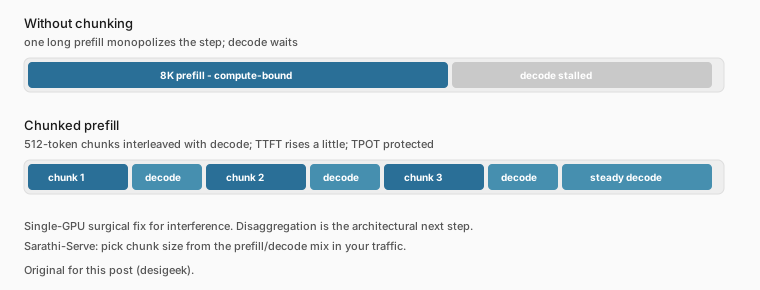
Two things on chunked prefill worth calling out - First, it is a scheduling compromise, not a cure. The same GPU is still doing both jobs; we have only time-sliced them so that no single prefill can grab a whole step. The interference between prefill and decode is smoothed, but the two phases still contend for the same silicon. Removing that contention outright means giving each phase its own hardware, which is disaggregation in section 5.
Second, chunked prefill gets cheaper the moment we pair it with prefix caching (the next section). The cost of a chunked prefill is basically the number of chunks it has to walk through, so anything that lets it skip chunks is a direct win. A cache hit on a shared prefix does exactly that: the chunks covering that prefix are already computed and get short-circuited, so a long prompt that is mostly a repeated system prompt ends up paying only for its unique tail. That shrinks the very TTFT penalty that made chunking a trade-off in the first place. vLLM’s Automatic Prefix Caching (APC) is what wires the two together.
1.5 Prefix caching
Many production workloads share a common prefix across nearly every request: the same system prompt, the same RAG document, the same few-shot examples. Recomputing the KV cache for that prefix on every request is pure waste. Prefix caching stores and reuses the computed KV cache blocks for token sequences the system has already seen.
SGLang’s RadixAttention is one of the cleanest implementations: it indexes KV cache blocks in a radix tree keyed on token sequences. A radix tree is a compressed prefix trie: each path from the root spells out a token sequence, sequences that start the same way share the same path until they diverge, and the tree branches only at the point where they differ. That shape is exactly right for prefix caching. A shared system prompt becomes a single trunk that every request hangs off, and working out how much of an incoming request is already cached is one walk from the root down to the point where the match stops. When a new request shares a prefix with a cached sequence, that walk is a cache hit, and the entire prefill for the matched prefix is skipped. vLLM calls its version Automatic Prefix Caching (APC). The math on what this saves is concrete.
Question: how many bytes of KV does one prompt token cost? For Llama-3.1-70B in FP16 with GQA (80 layers, 8 KV heads, head dim 128), multiply the five factors:
| Factor | Value | Why it is there |
|---|---|---|
| $n_{\text{layers}}$ | 80 | Every layer stores its own K and V |
| $n_{\text{KV heads}}$ | 8 | GQA: 64 query heads share 8 KV heads |
| $d_{\text{head}}$ | 128 | Elements per head |
| $2_{\text{K+V}}$ | 2 | Keys and values |
| $b$ | 2 | Bytes per element (FP16) |
$$ m_{\text{KV/token}} = n_{\text{layers}} \cdot n_{\text{KV heads}} \cdot d_{\text{head}} \cdot 2_{\text{K+V}} \cdot b $$ $$ m_{\text{KV/token}} = 80 \cdot 8 \cdot 128 \cdot 2 \cdot 2 = 327{,}680\ \text{bytes} \approx 320\ \text{KB/token} $$
Each factor is a real knob: fewer layers (smaller model), fewer KV heads (GQA/MQA/MLA), smaller $d_{\text{head}}$, or smaller $b$ (FP8 KV) all shrink $m_{\text{KV/token}}$. The model will differ, but the formula is the constant.
For a 4K system prompt, two numbers follow:
- First, the cache footprint of that prefix, its length times the per-token cost:
$$ M_{\text{KV}} = L \cdot m_{\text{KV/token}} = 4096 \times 320\ \text{KB} \approx 1.3\ \text{GB} $$
- Second, the latency it buys back. If a cold prefill of that prefix costs about 300 ms and roughly 90% of requests share it, the average TTFT we save is that cold-prefill cost scaled by the hit rate:
$$ \text{TTFT}_{\text{saved}} \approx 300\ \text{ms} \times 0.9 \approx 270\ \text{ms} $$
That 1.3 GB is what we avoid recomputing on a cache hit; with PagedAttention it is a block-table pointer share, not a memcpy. 😄
This is only possible because of PagedAttention. Without block-level KV management, prefix sharing would require copying gigabytes of data between requests. With paging, it’s a block-table pointer. The optimization lives entirely in the memory-management layer; no kernel changes are required.
This is also why API “cached input” prices sit far below fresh prefill: loading KVs beats recomputing them. It is the same $t_{\text{mem}}$ vs $t_{\text{compute}}$ split from Part 1, and it shows up in the COGS and on the price sheet.
1.6 Structured output breaks batch uniformity
Batching pays off because every sequence in a step runs the same matmul against the shared weights. That amortization holds regardless of what each request wants; what it quietly assumes is that the cheap work wrapped around the matmul (sampling, masking) is uniform across the batch too. Structured output is where that second assumption breaks.
The simplest example is a JSON schema. If the model is generating free-form text, every request in a batch can emit any token from the vocabulary at each step. If the model is generating structured output, some tokens are illegal at each step (e.g., closing braces before opening braces). The engine must mask those illegal tokens out of the logit vector before sampling, and that mask differs per request.
Structured/constrained decoding forces every emitted token to stay inside a schema (valid JSON, a regex, a grammar). Without it, clients parse free-form text and fail mid-stream; with it, the engine compiles the schema into a finite state machine and, at each decode step, masks illegal tokens.
The mask itself is cheap. The serving cost is that requests in one continuous batch sit at different FSM states, so their per-step masks differ and the decode step is no longer identical work across the batch. Keeping that fast enough to match unconstrained decoding is an active engineering problem, and structured-output throughput is now a first-class metric in vLLM, with xgrammar and llguidance the two dominant backends. Both are the engines that turn a schema into that per-step token mask: xgrammar compiles the grammar ahead of time and precomputes and caches the allowed-token masks so the hot path is close to a table lookup, while llguidance is a Rust engine that walks the grammar incrementally and computes the allowed-token set on the fly. Same job, different speed/flexibility trade-off; vLLM lets us pick.
1.7 Sampling isn’t free either
After each decode step the model emits a logit vector over the vocabulary; sampling turns that into the next token (temperature, top-k / top-p, then a draw). It is easy to treat this as free and model TPOT from weight and KV traffic alone, but at high concurrency that leaves our estimate optimistically low.
Take the simplest case: a 128K vocabulary, top-k=1, and a batch of 1,000 requests. Each request emits a logit vector of 128K floats (512 KB) and then samples one token. The sampling kernel must sort or partially reduce that 128K vector to find the top-k tokens for each request. That is a non-trivial amount of work, especially when we have thousands of requests in flight.
For a 128K vocabulary at large batch, that is a sort or partial reduction over a big tensor on every step, squarely in the decode critical path. At small batch it is noise; at high concurrency the sampling kernels become a measurable fraction of TPOT, which is why engines fuse them and why exotic settings (very large top-k, long logit-processor chains, per-request grammars) cost more than they look.
2. Quantization: fewer bytes per token
The engine decides how a request moves through the GPU; the next three sections decide how many bytes and tokens it costs. Quantization, multi-LoRA, and speculative decoding look unrelated, but each stretches one GPU across more useful work, and quantization is the most direct of the three. Decode is bottlenecked on bytes moved per token, so the lever is obvious: move fewer bytes per weight. That is quantization, representing model weights in lower-precision formats.
The table below lists bytes per weight and the theoretical decode-bandwidth gain that follows from it, treated as an upper bound. Realized throughput is always lower: it depends on the dequantization kernels and on whether the format runs natively on the tensor cores.
| Format | Bytes per weight | Theoretical decode bandwidth gain |
|---|---|---|
| FP32 | 4 | 0.5× (almost never used for inference) |
| BF16 / FP16 | 2 | 1× (baseline) |
| FP8 | 1 | ~2× |
| INT4 | 0.5 | ~4× |
| NVFP4 (FP4) | 0.5 | ~4× (native on Blackwell) |
For a 70B model in FP16 (140 GB), switching to INT4 (35 GB) means the GPU streams 4× less data per token. Plug that into the $T_{\text{mem}}$ formula from Part 1 :
$$ T_{\text{mem}}^{\text{INT4}} \approx \frac{35\ \text{GB}}{3.35\ \text{TB/s}} \approx 10.5\ \text{ms} $$
versus ~42ms in FP16. That is the theoretical bandwidth win. The realized end-to-end throughput for INT4 (AWQ, GPTQ) is typically 1.5 to 2.5×, because dequantization adds compute and INT4 doesn’t run natively on FP16/BF16 tensor cores. FP8 is closer to its theoretical 2× because it runs natively through the Tensor Cores: $b$ drops from 2 to 1, so $T_{\text{mem}}$ halves if nothing else changes.
2.1 Post-training quantization (PTQ)
Post-training quantization means we compress a finished checkpoint without a full retrain. We run a short calibration set, rewrite weights to fewer bits, and accept a small quality trade for a big memory and bandwidth win.
GPTQ (Frantar et al., 2022) and AWQ (Lin et al., 2023) are the two weight-only 4-bit recipes we will see most in production. Both aim to minimize output reconstruction error after quantization, but they take different approaches.
AWQ is currently preferred because it treats a small set of weight channels as special. A channel here is one slice of a layer’s weight matrix, the weights tied to a single input feature (picture one column).
Most channels are unremarkable, but a few are salient: the activations flowing through them are consistently large, so a rounding error in one of those channels swings the layer’s output far more than the same error somewhere quiet.
AWQ finds those channels from a short calibration pass and either keeps them at higher precision or rescales them before quantizing, which spends the accuracy budget where it actually moves the output. The result is significantly better quality at the same 4-bit budget. We don’t need to fine-tune the model; we only need a few hundred representative prompts to calibrate.
So far it looks like there are two knobs: the format (how many bits each weight gets) and, within a layer, which channels to protect. There is a third, and it matters as much as the other two: which layers to quantize at all. This is more than a yes/no we flip per layer, because quantization error has a sign. Rounding the weights in one layer nudges the model’s output one way; rounding a different layer nudges it back the other way. So the per-layer errors do not simply pile up, they can partly cancel, and choosing which layers to quantize can arrange for exactly that cancellation.
One team (Baseten) reported doing exactly this on GLM-5.2. By choosing which layers to quantize so their errors tended to cancel, they quantized more of the model than the stock recipes without the quality drop we would naively expect. This helped with higher throughput that comes from streaming fewer bytes. Whilst, we should treat this as one lab’s reported result rather than a principle, the underlying point is still interesting: quantization error interacts across layers, so which layers we quantize is a choice that matters, not just the format and the channels.
How they judged “no quality loss” is also interesting. Coarse benchmark scores are noisy (e.g. a two-point move on MMLU is usually run-to-run variance); instead they compared the quantized model against the full-precision one on a distributional metric: perplexity , which measures how confidently the model predicts held-out sequences token by token.
If perplexity barely moves, the quantized model is still placing its probability distribution on the same tokens as the original model. This is a better test of “we are serving the real model” than “it scored about the same on MMLU”, and helps catch the small drifts that only surface on the rare prompt where two candidate tokens are nearly tied, which is exactly where quantization quietly changes an answer.
2.2 FP8 and hardware-native paths
FP8 is where the hardware matches the format - specifically on Hopper (H100/H200) and Blackwell (B200/GB200), the tensor cores multiply in FP8 natively, so we skip the dequantize-then-BF16 tax that eats much of INT4’s theoretical win. That is why FP8 lands closer to a real 2× bandwidth story.
The catch is dynamic range: the gap between the largest and smallest numbers a format can represent. FP8 has only 8 bits, so that window is narrow. Cast a tensor into it naively and the values at the top overflow (they exceed the largest FP8 number and turn into garbage) while the values near zero underflow (they fall below the smallest FP8 number and get flushed to zero). Either way, information the layer needed is gone.
NVIDIA’s Transformer Engine is what makes FP8 safe despite that narrow window. The trick is scaling: before casting a tensor to FP8, it multiplies the whole tensor by a per-tensor scale factor chosen to slide that tensor’s actual range into the part of the FP8 window where the numbers are represented most accurately, does the matmul in FP8, then divides the scale back out while accumulating the result in BF16. Because it recomputes that scale factor per tensor, per layer, in hardware, each layer’s values are re-centered into FP8’s representable range on every pass, so nothing overflows at the top or vanishes at the bottom.
AMD solves the same problem the same way, just under different names: its Quark quantizer picks the scale factors and hipBLASLt runs the scaled FP8 matmul on the MI300X’s matrix cores (AMD also contributes a ROCm build of Transformer Engine itself, so the library often ports across). Either way, the mechanism is identical: scale in, matmul in FP8, scale out. This is not just a serving trick, either.
DeepSeek V3 was trained and served in FP8 natively, the first near-frontier model to do so at scale, and reported under 0.5% quality loss on standard benchmarks, which is what turned FP8 from a risky optimization into a default worth reaching for. By 2026 that default is visible on the shelf: open releases like Qwen3.8 (both the 27B and the 2.4T-A95B flagship) and GLM-4.5 ship an FP8 checkpoint next to the BF16 weights at launch, so FP8 serving is a download rather than a calibration project.
Blackwell pushes the same idea one precision lower. Its tensor cores multiply in FP4 natively, and the format we will meet in production is NVFP4, NVIDIA’s 4-bit floating-point layout with a small per-block scaling factor so that a group of weights shares one scale rather than trusting four bits to span the whole range on their own.
Because the multiply is native, FP4 skips the dequantize-to-BF16 tax that holds INT4 back, so it behaves much more like FP8 did on Hopper: close to the theoretical bandwidth win instead of half of it. The gains stack roughly by halving the format each step, but not by a clean 2× each: BF16 to FP8 buys on the order of 30 to 40%, and FP8 to FP4 buys a further 30 to 40% on top, so the full BF16-to-FP4 drop lands a bit under the naive 4× while being the single biggest bandwidth lever on a Blackwell box.
That is why “quantize to NVFP4” has become the default first move when a new OSS model lands, and why labs increasingly ship or calibrate an NVFP4 checkpoint alongside the BF16 weights (AMD’s MI355X does the same via the cross-vendor OCP MX formats, though the kernels and recipes land a little later on ROCm). 🤓
2.3 KV cache quantization
Weights and activations can be quantized separately from the KV cache. Quantizing the KV cache to INT8 or FP8 roughly halves its memory footprint, which enables longer contexts or larger batch sizes for the same GPU memory. vLLM exposes this with --kv-cache-dtype fp8. The precision loss is generally small, because KV values are averaged over many heads and layers before they contribute to the output.
Researchers are pushing well past that halving memory footprint. Together AI’s Kitty (MLSys 2026) drives the KV cache all the way down to 2-bit - but not uniformly. It identifies the key channels per head and keeps them at higher precision while quantizing the rest to 2-bit, a dynamic channel-wise boost that spends the bit budget where it actually matters. The net result is roughly an 8× smaller KV footprint for a reported quality loss under 0.5% on standard benchmarks.
2.4 Shrinking the KV cache at the source: GQA and MLA
Quantization shrinks the bytes per KV element. A parallel line of work shrinks the number of KV elements per token by changing the attention architecture itself. It is worth a look, because it is exactly why DeepSeek’s KV footprint looks nothing like the Llama numbers I used earlier: the Llama-3.1-70B GQA figure landed at ~320 KB/token, whereas DeepSeek’s MLA (the last stop below) drops the per-token cost to roughly 7% of a comparable MHA cache, so a DeepSeek token costs a small fraction of a Llama token to keep around.
Let us step back and start from what the KV cache actually holds. Attention runs as a set of parallel heads, and each head remembers a key (K) and a value (V) vector for every token it has already seen. That stack of stored K and V vectors is the KV cache, and it is exactly what decode has to stream out of HBM on every step.
More heads means richer attention but also a bigger cache. So the natural question is whether every head truly needs its own private K and V, or whether heads can share them. The four designs below form a spectrum, each a bolder answer to that one question than the last, and the whole spectrum works because those per-head vectors turn out to repeat a lot of the same information.
We should read them as steps along that spectrum - starting from where every query head keeps its own keys and values to heads sharing (or dropping) them ever more aggressively:
- Multi-Head Attention (MHA) gives every query head its own K and V. This means maximum quality, but also the largest KV cache.
- Multi-Query Attention (MQA) shares one K and V across all query heads. The cache shrinks by the head count, but also the quality suffers.
- Grouped-Query Attention (GQA) is the compromise in most modern dense models: query heads are split into a few groups, each sharing one K and V. That “8 GQA KV heads” figure from the prefix-caching math is exactly this: 64 query heads collapsed onto 8 KV heads, an 8× KV reduction at close to MHA quality.
Figure 6 lines the four variants up by how aggressively they share, or replace, KV heads. Each panel takes the same four query heads (Q1-Q4, grey) and shows how many stored KV heads (amber) they map onto. Fewer amber boxes means a smaller cache; MLA replaces them entirely with one latent (blue):

Multi-Head Latent Attention (MLA), introduced in DeepSeek V2 and carried through V3 and V4, attacks the problem from a different angle. GQA and MQA still store real K and V, just fewer copies of them. MLA stops storing them at all: it keeps one small latent vector per token and rebuilds the full K and V from it on the fly, trading a little extra compute each step for a much smaller thing to hold in HBM.
Two words in that sentence carry the whole idea: latent and low-rank. Let us take them one at a time.
A latent vector is a compressed stand-in, lossy like a JPEG rather than lossless like a zip file. Instead of storing the keys and values directly, MLA stores a shorter summary and rebuilds the full K and V from it whenever the layer needs them. Picture keeping a recipe card and cooking the dish on demand, rather than keeping a fully plated meal in the fridge for every token we have ever seen.
Low-rank is why that summary can be so much shorter without losing anything that matters. Start with how many numbers a token’s K and V actually hold: two (one for K, one for V), times the number of heads $n_h$, times the size $d_h$ of each head, which is $2 \cdot n_h \cdot d_h$ in all. That count is misleading, though, because the numbers are not independent: the heads carry a lot of overlapping information. The real content lives in far fewer dimensions than the raw count suggests, so a short latent of length $d_c \ll 2 \cdot n_h \cdot d_h$ can capture almost all of it. When the layer runs, a fixed linear map expands that latent back to full-size K and V. That is the whole trick: store the short summary, not the full K and V.
Concretely, MLA is just three matrix multiplies wired around the latent. Read them in the order the model runs them:
$$ c_{KV} = W^{DKV} h, \qquad K = W^{UK} c_{KV}, \qquad V = W^{UV} c_{KV} $$
The first multiply is the down-projection $W^{DKV}$. It runs once per token, squeezing that token’s hidden state $h$ into the short latent $c_{KV}$. That latent is the only thing written to the KV cache.
The other two are the up-projections $W^{UK}$ and $W^{UV}$. They run later, every time attention revisits this token, expanding the stored latent back into a full-size key and value on the spot.
So the split is clean: we pay the compression once and cache the result, then recompute the reconstruction each step from that one tiny vector. That is exactly the trade the section opened with, a little extra compute per step in exchange for a much smaller thing to keep in HBM.
The symbols, for reference:
| Symbol | Role |
|---|---|
| $h$ | Hidden state for this token (what the layer just computed) |
| $W^{DKV}$ | Down-projection: compresses $h$ into a short latent |
| $c_{KV}$ | Latent vector of length $d_c$, with $d_c \ll 2 \cdot n_h \cdot d_h$ (much smaller than full K+V) |
| $W^{UK}, W^{UV}$ | Up-projections: rebuild K and V during the forward, not from cache |
The payoff is what we no longer keep around. Only $c_{KV}$ lives in HBM, one short latent per token; the up-projections are ordinary weight multiplies folded into the forward pass, never cached. Compare footprints per token:
$$ m_{\text{KV/token}}^{\text{MHA}} \propto 2 \cdot n_{h} \cdot d_{h}, \qquad m_{\text{KV/token}}^{\text{MLA}} \propto d_{c} $$
Since $d_c \ll 2 n_h d_h$, the MLA side is far smaller, and that gap is the whole point. DeepSeek V2 reported a 93.3% reduction in KV cache, down to roughly 7% of the pre-MLA size, well past what GQA delivers. It gave up no quality doing so, matching or beating MHA on DeepSeek’s own evaluations.
To see why that matters, tie it back to the decode math from Part 1 . The KV traffic term there is $B \cdot L \cdot m_{\text{KV/token}}$: it grows with batch size $B$, sequence length $L$, and the per-token cost. Shrink $m_{\text{KV/token}}$ and that term grows more slowly, so we can pack a larger $B$ into the batch before KV traffic eats the free lunch batching was buying us.
None of this is free, though. MLA runs straight into RoPE (Rotary Position Embedding), the standard way a model encodes where each token sits: it rotates every key and query vector by an angle set by the token’s position in the sequence.
The challenge though is that RoPE expects a full-size key to rotate, and MLA never keeps one around, it keeps the latent, so at cache time there is nothing for the rotation to act on. DeepSeek’s fix is decoupled RoPE: a small slice of each key skips the compression and carries the rotary position uncompressed, while the rest goes through the latent path. Someone has to wire that split in by hand in the serving layer, which is exactly why solid MLA support in vLLM and SGLang trailed the model releases by months.
And that lands us back on the same chain as the rest of this section: a smaller KV cache per token means more tokens fit in the same memory budget, which means larger decode batches, which means one weight read amortizes across more tokens in flight. MLA is just another route to that destination, pulling decode back toward the compute-bound side of the roofline.
The newer frontier: linear-attention hybrids. MLA is the end of the shrink the KV cache line, but the 2026 frontier models take a different exit entirely: they stop keeping a per-token KV for most layers at all. Qwen3-Next and the Qwen3.8 family (both the 27B dense model and the 2.4T-A95B flagship) interleave Gated DeltaNet, a gated linear-attention layer, with periodic full Gated Attention, in a repeating pattern of roughly three linear layers to one full-attention layer. A linear-attention layer replaces the growing key/value stack with a fixed-size recurrent state: it folds each new token into a constant-size summary of the past instead of appending to a cache that grows with context. The same idea powers the broader state-space family (Mamba and its successors).
That changes the decode physics this whole section is built on. For a linear-attention layer the KV-per-token cost is not shrunk, it is gone: memory and per-step work do not grow with sequence length, which is exactly how these models advertise 256K to 1M context cheaply. The catch is that a fixed-size state is lossy, it cannot attend to an arbitrary past token exactly, so the models keep a few full-attention layers in the mix to preserve exact long-range recall. That is why they are hybrids, not pure linear models, and why the KV-cache math above still matters, just for a minority of layers. Read the spectrum this way: GQA and MLA shrink the KV cache; linear-attention hybrids delete it for most of the stack and keep full attention only where exact recall earns its cost.
2.5 A note on determinism
One consequence of everything in this section (and the kernel sections before it) that surprises most is that the same prompt at temperature 0 can produce different outputs at different batch sizes, or across engine versions, or between quantization settings.
The root cause is one property of floating-point math: addition isn’t associative, meaning $(a + b) + c$ can differ from $a + (b + c)$ in the last bits. A float has only so many significant digits, so adding a large number to a tiny one rounds part of the tiny one away; do the tiny ones first and they survive enough that they nudge the result.
A matmul is millions of such adds, and the batch size changes which kernels run, how those reductions are tiled, and in what order the partial sums accumulate; as one would expect the last bits of each logit shift. Usually this doesn’t matter and is invisible, but when two candidate tokens are nearly tied, a shift in the last bits can determine which one wins, and then the whole generation diverges from there. FP8 tightens the numerics further, so tiny differences cross those token-selection boundaries more easily.
None of this is a bug in any individual layer; it’s the same leak as the dtype story: kernel-level details show up through abstractions that look transparent. If our product or evaluation pipeline assumes bit-identical reproducibility, we have to pin far more than the model weights: engine version, kernel backends, quantization config, and even the batching regime.
All of this floating-point rounding whilst annoying is the benign cause. There is a much nastier cousin that is a genuine concern: a race condition inside a kernel, of the kind Part 2 flagged. A hand-written kernel with a missing or mis-placed barrier can let some threads read a value before other threads have written it, and whether that misfires depends only on the order the hardware happened to schedule its warps.
The most interesting way this shows up in production: the same weights, on the same engine, will collapse into repeating a single token (a mode collapse, often the letter “S” or a run of dashes) on one cluster and behave perfectly on another.
The difference turns out to be the interconnect: the fabric wiring the GPUs together, NVLink between the cards inside one node and InfiniBand or RoCE between nodes (the same links the disaggregation section leaned on for KV handoff). Its only job is to move bytes between GPUs, but how fast it moves them sets the relative timing of everything downstream. On the slower cluster, the node-to-node KV-cache transfer takes long enough to shift that timing, and the shift exposes a race the faster cluster’s timing happened to hide. No weight is wrong and no quantization is wrong; the same bytes just arrive in a different order.
Teams end up pinning the model to the cluster that does not trigger it while they chase the missing barrier upstream (frequently the fix is pulling in a newer TensorRT-LLM or vLLM kernel image). It is the determinism version of this series’ opening bug: a contract living inside a C++ kernel that nothing above it can see.
3. Serving many fine-tunes: multi-LoRA
How many variants of one base model can we serve on a single GPU without dedicating hardware to each? That is the multi-LoRA question, the one I keep hearing about from customers. It sits naturally beside quantization: both stretch one GPU across more useful work, one by shrinking the weights, the other by sharing a base across many fine-tunes.
This section is about serving many fine-tunes; making them is a book in its own right. That is exactly what my new book📘, LLM Customization and Fine-Tuning: Adaptation, Distillation, and Alignment , is about: LoRA and QLoRA, full supervised fine-tuning, distillation, and DPO alignment, each carried end to end on a single GPU. It is in Early Access ( MEAP ) from Manning now.
A team fine-tunes a base into dozens or hundreds of task-specific or customer-specific variants with LoRA (Low-Rank Adaptation): small trainable matrices inserted into a frozen base. Each adapter is typically tens to a few hundred MB; the base is tens of GB. Serve them naively (load adapter A, handle its traffic, swap to adapter B), and the whole fleet runs one adapter at a time, with every other adapter’s requests waiting for the swap. The trick is keeping the base resident and batching across adapters in one forward pass.
3.1 How LoRA adapters work
A LoRA adapter is a tiny trainable adapter that sits on top of a frozen base weight. The base model doesn’t change; instead, next to each big weight matrix $W$ we keep two thin matrices, $A$ and $B$, and their product stands in for the adjustment that fine-tuning would have made.
Because those two matrices are small, an adapter is tens of MB in size while the base stays tens of GB, so a single GPU can hold the base once and swap only the little adapter in and out. At run time the math splits in two: a shared base multiply that every request runs against the same $W$, plus a small adapter-specific step layered on top. That split is the detail that later lets many adapters ride in one batch.
Why can two skinny matrices stand in for a full weight update? The answer is the low-rank idea in the name, the same one that kept MLA’s latent small, reused here for a different tensor. Picture the update as a $d \times k$ grid: in principle a fine-tune could rewrite every one of those $d \cdot k$ numbers independently. In practice it does far less. Fine-tuning nudges the weights along only a small handful of directions, not all $d \times k$ of them at once. The rank $r$ is simply how many of those directions we choose to keep, and it is tiny (16 is a common value).
Those two thin matrices are how we pin the update to just $r$ directions. Written as $B A$, a $d \times r$ matrix times an $r \times k$ one, the product can only reach $r$ directions and no more, so we keep those instead of the whole grid. Where MLA compressed the KV cache into a short latent, LoRA compresses the weight update into this low-rank pair: same trick, different tensor.
Written out, for a frozen base weight $W_0 \in \mathbb{R}^{d \times k}$ (that is $d$ rows and $k$ columns), the adapted weight is the original plus the low-rank update:
$$ W = W_0 + \Delta W = W_0 + BA $$
where $B \in \mathbb{R}^{d \times r}$ and $A \in \mathbb{R}^{r \times k}$, with the rank $r$ far smaller than either dimension ($r \ll \min(d, k)$). The saving is just a matter of counting entries. The full matrix $W_0$ carries one number for every (row, column) pair, so $d \cdot k$ of them. The thin pair carries far fewer: $B$ holds $d \cdot r$ entries and $A$ holds $r \cdot k$, which add up to $r(d + k)$.
$$ N_{\text{params}}(W_0) = d \cdot k, \qquad N_{\text{params}}(BA) = r(d + k) $$
Since $r$ is small (again, think 16) while $d$ and $k$ run into the thousands, replacing $d \cdot k$ with $r(d + k)$ cuts the parameter count by two to three orders of magnitude. That is the whole reason an adapter is a few tens of MB against a base of tens of GB.
To make it concrete: a rank-16 adapter on Llama-3-70B is about 80 MB, against 140 GB for the FP16 base, roughly a 1,750× size ratio (assuming the adapter touches the query and value projections at all 80 layers in FP16). The exact ratio moves with the rank and with which modules we adapt; against an INT4 base (35 GB), the same adapter lands closer to 437×.
The forward pass separates cleanly:
$$ y = W_0 x + B(Ax) $$
The two terms just add. $W_0 x$ is the shared base matmul, identical for every adapter in the batch. $B(Ax)$ is the adapter’s correction: $Ax$ compresses the activation down to rank $r$, then $B$ expands it back, and only this second term depends on which LoRA a request loaded. That additivity, no cross-terms tangling the two together, is the whole trick: we run the base matmul once for the entire batch and layer each request’s small adapter term on top. Figure 7 is the mixed-batch picture:

3.2 Batching across adapters
S-LoRA (Sheng et al., MLSys 2024) and Punica (Chen et al., MLSys 2024) are the two research serving systems that first cracked the mixed batch, and it is worth seeing what made it hard. The goal is one batch in which different requests want different adapters: row 1 is running on adapter A, row 2 on adapter B, row 3 on C. Tag each row with the adapter it loaded and the forward pass from 3.1 picks up a per-request index $i$: request $i$ computes $y_i = W_0 x_i + B_i(A_i x_i)$. That is the same two-term split as before, but the two terms now behave very differently under batching.
The base term $W_0 x_i$ is the easy one. The frozen base $W_0$ is shared by every request no matter which adapter it loaded, so all the rows stack into one big matmul, exactly the batching the base model already gets.
The adapter term $B_i(A_i x_i)$ is the troublemaker, because $A_i$ and $B_i$ change from row to row: row 1 multiplies by adapter A’s matrices, row 2 by adapter B’s. An ordinary matmul assumes one shared weight for the entire batch, so it has no way to say “row 1 uses adapter A, row 2 uses adapter B.” The naive fallback is to loop over adapters one at a time, but that serializes the batch and throws away the win we were after.
Their fix is a grouped GEMM. A GEMM (general matrix multiply) is just the standard dense matrix-multiply kernel a GPU is built around; the grouped version runs many of them in one shot, applying a different small matrix to each group of rows in a single fused kernel launch. So every adapter’s delta path runs together in that one op, sitting beside the shared base matmul, and a batch of mixed adapters stays about as efficient as a uniform one. It is the same class of kernel that MoE expert dispatch uses (different small expert matrices, one launch), which is why LoRA serving and MoE routing keep showing up side by side. Figure 8 puts the naive loop and the grouped GEMM side by side:

vLLM supports this out of the box and is enabled using two flags:
--enable-loraswitches the adapter path on at all, so the server will accept a LoRA name per request and add the adapter term to the forward pass.--max-lorasthen caps how many distinct adapters may be live in GPU memory within a single batch: set--max-loras 8and up to eight different adapters can ride one grouped GEMM together, while a ninth request waits for a slot. (A companion flag,--max-lora-rank, sizes those $A$/$B$ matrices for the largest rank we plan to serve.) We keep the pool small because each resident adapter costs GPU memory and widens the grouped GEMM; we keep it larger than one so mixed traffic actually batches.
Adapters beyond that live cap are not lost, just not resident: they sit in CPU RAM and get swapped into a GPU slot on demand when a request asks for them, the same paging idea PagedAttention uses for KV blocks, now applied to adapter weights. That swap is what lets the registered library dwarf the live cap. With S-LoRA, a single server can register thousands of distinct LoRA variants and page them through a handful of GPU slots, serving all of them without dedicating capacity to any one, which is the whole reason this lever sits beside quantization in the byte/token economy.
4. Speculative decoding
Quantization and multi-LoRA both shrink what a request has to move; speculative decoding runs the trick in reverse, buying several tokens from a single weight load instead of shrinking bytes. It is the last of these single-GPU levers, needs no infrastructure changes, runs on a standard serving setup, and is mathematically lossless.
4.1 The core insight
As we saw in Part 1, decode steps are expensive because each one reloads weights from HBM and is therefore bandwidth-bound. Speculative decoding buys multiple output tokens per target forward by exploiting a structural asymmetry: autoregressive generation is sequential; verification over a short candidate window is parallelizable over positions and reuses one weight load.
Why is verifying cheaper than generating? Generating token $t+1$ needs token $t$ to exist first, so we pay one full weight read per token, strictly one at a time. Verification has no such dependency, because the candidate tokens are already sitting there, proposed by the draft. We can lay all $K$ of them out as one input sequence and run a single target forward that scores every position at once, checking “given the first $i$ candidates, what would I have produced at position $i+1$?” for all $i$ in parallel. That forward reads the target’s weights from HBM exactly once, the same read a single decode step already pays, and decode is bandwidth-bound, so folding $K$ positions into it is nearly free: the weight traffic is unchanged and only a little extra math rides along. One weight read now adjudicates $K$ tokens instead of producing one.
We can verify a $K$-token draft in one target forward for roughly the cost of verifying one token. The algorithm, from Leviathan et al. (Google, ICML 2023) and Chen et al. (DeepMind, 2023), runs as follows:
- A small draft model generates K candidate tokens autoregressively, recording its probability distribution $q(\tilde{x}_t)$ at each step
- The large target model runs one forward pass over all K candidates simultaneously, producing its distribution $p(x)$ at each position
- Accept or reject left-to-right: draw $u \sim \text{Uniform}[0, 1]$; accept $\tilde{x}_t$ if $u \le p(\tilde{x}_t) / q(\tilde{x}_t)$
- On rejection at position $t$, sample a corrected token from $\text{normalize}(\max(0, p(x) - q(x)))$ and stop
- If all K tokens are accepted, sample one bonus token from the target’s distribution at position K+1
Figure 9 is the algorithm as a flowchart; Figure 10 is Google Research’s animation of the same idea (accepted tokens in green, rejected in red):

It pairs cleanly with a cheap draft against a heavy target (quantization), and with Flash-Decoding on long contexts.
4.2 Why this is lossless
The acceptance-rejection rule in step 3 is a well-known technique from statistics called rejection sampling. The key property is that regardless of what the draft model produces, the accepted token sequence has the same marginal distribution as if the target model had generated it directly, token by token. There’s no approximation. The output distribution is exactly $p$, for every token, every time.
We can verify this by working through the marginal: at any position, the probability of the accepted token being $x$ integrates out the draft’s proposal and recovers $p(x)$ exactly. The corrected token in step 4 ensures that even on a rejection, the fallback token is correctly distributed under $p$.
4.3 Expected speedup
Whether speculation earns its place comes down to one question: across a single draft-and-verify round, do we keep enough tokens to pay for the draft we ran to get them?
Answering this is a two-step calculation, first the tokens we expect to keep, then those tokens weighed against the round’s cost. We can break it down with three measurable quantities:
| Symbol | Meaning |
|---|---|
| $\alpha$ | Mean acceptance rate: fraction of draft tokens the target agrees with |
| $K$ | Draft length: how many tokens the draft proposes per round |
| $c$ | Cost ratio: draft step cost ÷ target step cost (e.g. 0.1 if the draft is ~10× cheaper) |
The first two, $\alpha$ and $K$, are the knobs we actually tune; $c$ is fixed by how cheap our draft model is to run, meaning how little time one of its decode steps takes next to the target’s. A draft with far fewer parameters streams far fewer bytes from HBM per step, so it lands a small $c$ (0.1 says a draft step costs a tenth of a target step). Higher $\alpha$ raises the tokens we get per target forward, while higher $K$ helps only for as long as acceptance stays high and the draft stays cheap, a tension the math below makes exact.
Step 1: how many tokens we keep per round. Acceptance runs left to right and stops at the first reject, so keeping the third token requires the first two to have passed too, keeping the fourth requires the first three, and so on down the draft. Each further token we hold onto is therefore less likely than the one before it, which is why the contributions decay as powers of $\alpha$ instead of staying flat.
Model each draft position as accepted independently with probability $\alpha$: we always keep the first attempt (contribution $1$); with probability $\alpha$ we also keep the second (contribution $\alpha$); with probability $\alpha^{2}$ the third; and so on through $K$ draft tokens. If all $K$ pass, the target also emits one bonus token (contribution $\alpha^{K}$). So the expectation is the finite geometric series:
$$ \mathbb{E}[\text{tokens per pass}] = 1 + \alpha + \alpha^{2} + \cdots + \alpha^{K} = \frac{1 - \alpha^{K+1}}{1 - \alpha} $$
(The closed form is the usual sum $S = (1-r^{n})/(1-r)$ with $r=\alpha$ and $n=K+1$ terms.)
Note: A worked check is just that: plug real numbers into the formula and confirm it lands where the reasoning says it should, a habit worth keeping for anything we are going to rely on.
For $\alpha=0.8$, $K=4$, expand the series first, then use the closed form and see the two agree:
$$ 1 + 0.8 + 0.64 + 0.512 + 0.4096 = 3.3616 $$
$$ \frac{1 - 0.8^{5}}{1 - 0.8} = \frac{1 - 0.32768}{0.2} = \frac{0.67232}{0.2} = 3.36 $$
Same answer two ways. One target forward yields ~3.4 output tokens instead of 1. Table for other $(\alpha, K)$:
| Mean acceptance rate $\alpha$ | Draft tokens K | Expected tokens per pass |
|---|---|---|
| 0.7 | 4 | 2.77 |
| 0.8 | 4 | 3.36 |
| 0.9 | 4 | 4.10 |
| 0.9 | 8 | 6.13 |
| 0.95 | 8 | 7.40 |
Step 2: turn tokens kept into wall-clock speedup. That expectation counts tokens per round, which is not yet a speedup. The round was not free: we ran $K$ draft steps to propose those tokens before the target ever looked at them. So the honest measure is what we gained divided by what we paid.
Call the expectation from step 1 $E$. That is the gain, the tokens we keep. The cost is the whole round measured in target-step equivalents: one full target verify, plus the $K$ draft steps, each counting as only a fraction $c$ of a target step. Put gain over cost:
$$ \text{speedup} \approx \frac{E}{1 + K \cdot c} $$
Worked check: $K=4$, $c=0.1$, $\alpha=0.8$ so $E=3.36$:
$$ \text{speedup} \approx \frac{3.36}{1 + 4 \cdot 0.1} = \frac{3.36}{1.4} \approx 2.4\times $$
Read that 2.4× as one target forward now delivering what used to take almost two and a half of them, with the draft’s cost already subtracted out. The whole result hangs on the denominator: if $\alpha$ drops (the target rejects more of the draft) or $c$ rises (the draft gets relatively more expensive), the denominator grows against $E$ and the speedup shrinks, and can even fall below 1, at which point speculation is costing us rather than helping. That is why production turns it on for latency-sensitive, lightly loaded decode and turns it off once the GPU is already batch-bound. Some of the variants in 4.4 attack the same denominator by amortizing the draft cost differently, and some systems overlap draft and target execution.
Real production numbers for code-generation workloads, where draft acceptance rates are high because code follows predictable patterns, land around 2 to 3× on end-to-end throughput.
That code-generation number is not an accident, and it points at the most important operational lever in speculation: the draft is only as good as its match to our traffic. The acceptance rate $\alpha$ is not a property of the target model alone; it is a property of how well the draft predicts the tokens our users actually ask for.
Code is highly predictable (boilerplate, closing brackets, repeated identifiers), so a draft trained on code earns a high $\alpha$ and a large speedup. Point that same draft at open-ended prose and $\alpha$ falls, and the speedup falls with it. So the strongest deployments train a custom speculator on their own traffic distribution: a coding provider trains its draft on code, an agent platform on tool-call and JSON-heavy transcripts.
There is a catch here that ties speculation back to the rest of the stack. The draft has to be trained against the target’s own hidden states, so building one needs the real target weights plus prompts representative of our traffic, which means a traffic-specific speculator only makes sense on a dedicated deployment.
A shared, multi-tenant API cannot offer one, because it has no idea whether the next request is code, a legal brief, or a summary of every Harry Potter book, so it falls back to a general-purpose draft with a lower average $\alpha$. This is one of the concrete reasons high-volume users graduate from a shared token API to renting the box: on their own hardware they can train a speculator that knows what their traffic looks like.
Two limits bound all of this, and both are worth stating plainly. Speculative decoding only accelerates decode: prefill still runs at full price, so if our bottleneck is TTFT (common for interactive apps with long prompts), speculation does nothing for it. And at high batch sizes it often turns negative, because the draft steals FLOPs and VRAM from an already-saturated target GPU, so the speedup math above, which quietly assumes the target has headroom to spare, stops holding.
4.4 Variants
The base algorithm assumes a separate draft model. Production systems often change who proposes the tokens, or how acceptance is tuned to the traffic, because managing a second model is awkward. Draft quality varies a lot by domain. Four variants we will hear about:
Medusa (Cai et al., 2024): instead of a separate draft model, attach multiple prediction heads directly to the target model, so head 1 predicts $t+1$, head 2 predicts $t+2$, and so on. The heads run in parallel alongside the main forward pass, adding minimal overhead. Acceptance rates are lower than for a well-matched separate draft model, but there’s no separate model to manage or load.
EAGLE (Li et al., 2024): the draft model operates on the target model’s internal feature vectors rather than its output token embeddings. Because it works in the target’s own representation space, it gets dramatically higher acceptance rates, typically 0.85 to 0.93 versus 0.65 to 0.8 for conventional draft models.
Distribution-Aware Speculative Decoding (DAS) (Together AI, MLSys 2026): during RL training rollouts, token distributions are highly non-uniform, with certain tokens appearing far more often in rollout trajectories than others. DAS adapts the draft length dynamically based on the measured distribution of the current training batch, achieving up to 50% faster RL rollout throughput with zero reward-quality degradation. This is the connection between inference serving and the training pipeline that produces reasoning models.
DSpark (DeepSeek, 2026): DeepSeek’s own successor to static MTP, and the clearest sign of where this is heading. It pairs a semi-autoregressive draft (a heavy parallel backbone plus a lightweight sequential head that injects intra-block dependency, curing the acceptance decay that pure parallel drafters hit late in a block) with confidence-scheduled verification: a small confidence head estimates each draft token’s survival probability, and a load-aware scheduler sets the verification length per request, spending target-model batch capacity only on tokens likely to be accepted. Deployed in the DeepSeek-V4 serving system it replaced the MTP-1 baseline and reported 60 to 85% faster per-user generation at matched throughput, precisely by not wasting verification on low-confidence suffix tokens under high concurrency. This is where speculation (section 4) meets the fleet scheduler (section 7): the draft length becomes a per-request scheduling decision rather than a fixed knob.
4.5 When the draft is baked into the model: MTP
Everything above adds speculation to a model after the fact. DeepSeek V3 and V4 take the opposite approach: the drafting capability is trained into the model itself, through Multi-Token Prediction (MTP). During training, extra prediction heads sit on top of the main model so that head 1 learns to predict $t+1$, head 2 predicts $t+2$, and so on, sharing the output embedding and trained with losses that taper as training matures. At inference, those heads become a built-in draft path: the main model proposes the next token, the MTP heads propose the following few, and a single verification pass accepts or rejects them.
The reason this beats an external draft model is the same reason EAGLE does. The MTP heads live in the model’s own representation space and were trained jointly with it, so their proposals line up with what the main model would have produced, and acceptance rates are correspondingly high. SGLang shipped MTP as a plug-and-play option for DeepSeek in 2025 and reported immediate decode speedups.
MTP is no longer a DeepSeek-only trick, and that spread is the real signal. It has become close to a default across open models. In the Qwen family it now runs the whole size range: Qwen3.8 trains in MTP from the flagship 2.4T-A95B MoE down to the compact dense 27B vision-language model small enough to run on a workstation (the earlier Qwen3-Next already carried it). The GLM line does the same and keeps pushing it: GLM-4.5 and GLM-4.6 shipped an MTP layer that doubles as an EAGLE-style speculative head, and the current flagship GLM-5.2 improved that MTP head specifically for speculative decoding, reporting up to 20% higher acceptance length. Once independent labs bake the draft into the architecture across everything from trillion-parameter MoEs down to a 27B dense model, trained-in speculation stops being an optimization we add after the fact and becomes part of how the model ships.
That ubiquity makes one practical check worth stating: a model with MTP in its name is not proof MTP is doing anything. Confirm the engine actually initializes the speculator (the launch flags decide this, not the checkpoint), and read the acceptance rate off the serving logs, which is the \alpha from 4.3 measured on our own traffic rather than assumed. To turn it into a speedup headline, A/B against the same weights with the MTP path disabled, holding hardware, engine version, prompt, and sampling fixed, and report median tokens/s and TTFT next to the acceptance rate.
For someone deploying DeepSeek V4-Pro, MTP is a real operational lever rather than a footnote. To size it, the reference case is DeepSeek V3: its MTP module was roughly 11.5B parameters, about 1.7% of that 671B model, and V4-Pro carries the same design at its own larger scale. Keep the heads, and we get a native 1.5 to 2× decode speedup with no separate draft model to manage; strip them, and we reclaim that weight loading and memory for a purely throughput-bound, memory-constrained deployment. Those same heads ride the fused MoE path the opening bug lived in: architecture choices show up as serving contracts. 😏
5. Disaggregating prefill and decode
Every lever so far has kept prefill and decode on the same GPU and squeezed more out of that shared silicon. This is the section where the two finally split apart. Chunked prefill only mitigates the interference between them; it never removes it, because the same GPU is still doing both jobs. The only way to remove it outright is to stop sharing: run prefill on one set of machines and decode on another, so a compute-bound prompt pass can no longer stall a bandwidth-bound decode and blow its SLO. That is disaggregation, and the price of admission is handing the KV cache from one pool to the other mid-request.
The DistServe paper (Zhong et al., OSDI 2024) quantifies what happens to TPOT under bursty workloads with colocated serving: P99 TPOT can exceed SLO targets by 10 to 30× when a wave of long-prompt requests arrives (on their benchmark setup). The underlying issue is that meeting TTFT SLOs requires provisioning for peak prefill throughput, while meeting TPOT SLOs requires provisioning for peak decode throughput, and these have different optimal batch sizes, different parallelism strategies, and different memory footprints. Trying to serve both from the same pool of GPUs means constantly compromising both.
5.1 The disaggregation architecture
Prefill workers own the compute-bound prompt pass; decode workers own the bandwidth-bound token stream; a router hands the request across after prefill. The hard constraint is KV transfer: a few thousand prompt tokens can be >1 GB of state that must cross the fabric inside the TTFT budget, which is why InfiniBand, RDMA, and NVLink show up in every serious design. RDMA (Remote Direct Memory Access) is the property that makes this affordable: one machine’s network card writes straight into another machine’s memory without either CPU copying the bytes or the kernel’s TCP stack touching them, so a multi-GB KV cache moves at close to raw wire speed instead of being throttled by host software.
Split the serving fleet into two pools:
- Prefill workers: receive new requests, process the full prompt in one (or few) forward passes, produce the initial token plus a complete KV cache
- Decode workers: receive the KV cache from prefill workers, take over the request, stream tokens until completion
A router sits in front, directing new requests to available prefill workers and routing the handoff to decode workers. Each pool scales independently based on its own utilization. Figure 11 is the architecture:

The hard engineering problem is the KV cache transfer. A 4K prompt on Llama-3.1-70B in FP16 produces about 1.3 GB of KV cache (~320 KB per token). In a disaggregated setup, that same 1.3 GB now has to cross the network between the prefill worker and the decode worker. Transfer time is just size over sustained bandwidth:
$$ T_{\text{xfer}} = \frac{M_{\text{KV}}}{B_{\text{net}}} $$
Budget example. Target TTFT 500ms, prefill already uses 200ms, so the handoff gets a 300ms budget:
$$ B_{\text{net, min}} = \frac{1.3\ \text{GB}}{0.3\ \text{s}} \approx 4.3\ \text{GB/s} $$
Round up for protocol overhead and we want roughly ≥4.5 GB/s sustained to clear one request’s KV inside the handoff budget. Here is what each common fabric actually delivers against that bar:
| Network | Bandwidth | $T_{\text{xfer}}$ for 1.3 GB |
|---|---|---|
| 25GbE | 3.1 GB/s | ~420ms (not viable) |
| 100GbE | 12.5 GB/s | ~104ms |
| InfiniBand HDR (200Gb) | 25 GB/s | ~52ms |
| RoCEv2 / RDMA over 100GbE | ~12 GB/s effective* | ~108ms |
| NVLink (intra-node) | 600 GB/s | ~2.2ms |
RoCEv2 and InfiniBand RDMA bypass kernel TCP stacks and cut CPU overhead on KV handoffs. Raw line rate on 100GbE looks fine on paper; without RDMA, latency jitter and host CPU load often blow tight TTFT budgets in production.
This is why disaggregation requires high-speed interconnect infrastructure: we can’t run it over a commodity Ethernet network and still meet tight TTFT SLOs.
Prefix sharing changes the transfer story. When many concurrent requests share a 4K system prompt, a decode worker that already holds that prefix in cache (via APC or LMCache) can skip the transfer entirely for the shared portion. Only the request-specific suffix needs a prefill handoff. At scale, this is why systems like LMCache and Mooncake invest in cross-worker KV cache affinity and reuse, not just raw transfer bandwidth.
Let us double click on three things we called out in that last sentence:
- KV affinity (per-session pinning) is a routing property: a follow-up request lands back on the worker that already holds its KV cache, so the history it built up is reused rather than recomputed, and losing it means every turn re-prefills from scratch.
- LMCache is an OSS KV cache layer that bolts onto vLLM or SGLang and moves KV blocks out of GPU memory into a tiered store (CPU RAM, local SSD, remote backends), so a cache that no longer fits in HBM spills instead of being discarded, and the same blocks can be reused across requests, sessions, and separate engine instances.
- Mooncake (Moonshot AI) takes that idea to a disaggregated fleet: a shared, cross-worker KV store that lets any decode worker pick up a prefix another one already computed. LMCache and Mooncake both exist for the same reason: past a certain scale, the KV cache earns its keep as a managed storage tier rather than scratch memory that dies with the request.
5.2 Production systems
The research papers established the prefill/decode (P/D) split; production systems turned it into a control plane and a KV transfer path. The two names to know are NVIDIA Dynamo (a full-stack framework with NIXL worker-to-worker KV writes) and llm-d (the same architecture built on Kubernetes Deployments and HPAs), and both map this design onto how most fleets already run.
The table below collects the headline results from the papers and vendors that built these systems. Read each figure as what that author measured on their own setup, not a transferable ranking.
| System | Key result | Venue |
|---|---|---|
| DistServe (Zhong et al.) | 7.4× more goodput, 12.6× better SLO attainment | OSDI 2024 |
| Splitwise (Microsoft Research) | 2.35× throughput at same cost | ISCA 2024 |
| Mooncake (Moonshot AI) | 525% throughput improvement | FAST 2025 (Best Paper) |
| SGLang R1 production (DeepSeek) | 52.3K input tokens/s, 22.3K output tokens/s on 96 H100s | public benchmark |
NVIDIA Dynamo (GTC 2025, open-sourced) is NVIDIA’s disaggregated serving framework, and it is worth walking through because it shows how the abstract P/D split turns into a real system. Its one load-bearing idea, taken straight from Dynamo’s architecture docs, is that there is no shared KV cache store: the decode worker pre-allocates the KV blocks first, and the prefill worker RDMA-writes its result straight into them, worker to worker. That direct write is exactly what earlier disaggregation prototypes got wrong, routing KV through a central store that then became the bottleneck. The path below traces one request through that design, and each hop reuses a piece we have already built:
- Frontend, the front door. It speaks the OpenAI-compatible HTTP API, tokenizes the prompt, applies the chat template, and hands the request to a decode worker. Note the twist: the request lands on the decode side first, not prefill, and step 2 is why.
- The decode worker reserves the room before the guest arrives. It first checks its own prefix cache, the fleet-wide version of prefix caching from section 1.5, so any prefix it already holds is not recomputed. For the rest of the prompt it makes the disaggregation decision: it pre-allocates, in its own HBM, the KV blocks the answer will eventually live in, then requests a remote prefill that names those block IDs. This is the crux of the whole design. Because the decode worker owns the destination up front, the prefill worker later has a fixed address to write into, and no shared store ever sits in the middle.
- A durable queue hands the prefill to whoever is free. The request waits in a prefill queue, and any idle prefill worker claims it. This is plain load-balancing: it separates a prefill is needed from which GPU runs it, which is what lets the two pools scale independently.
- The prefill worker does the heavy pass and writes straight into decode’s memory. It looks up the decode worker’s pre-allocated block addresses, runs the prompt through the model (the compute-bound TTFT work from Part 1 ), and RDMA-writes the resulting KV cache directly into those blocks through NIXL, NVIDIA’s transfer library that hides NVLink, InfiniBand, PCIe, and NVMe behind one block-based API. No staging buffer, no CPU copy: the bytes leave the prefill GPU and land in the decode GPU’s KV cache. And these are the very same PagedAttention blocks from section 1.2, only now they cross the fabric instead of living inside one GPU.
- The decode worker takes over and streams. The write lands at the addresses it chose back in step 2, so its KV cache is already populated and it just starts decoding (the bandwidth-bound TPOT work) and streams tokens back out through the Frontend.
In Dynamo’s implementation the durable queue is NATS JetStream and the coordination store is etcd, but neither choice is load-bearing: any durable queue and any coordination store would fill the same roles. What matters is the shape of the handoff, pre-allocate, dispatch, RDMA-write, decode.
As a sequence, the write-back path looks like Figure 12:
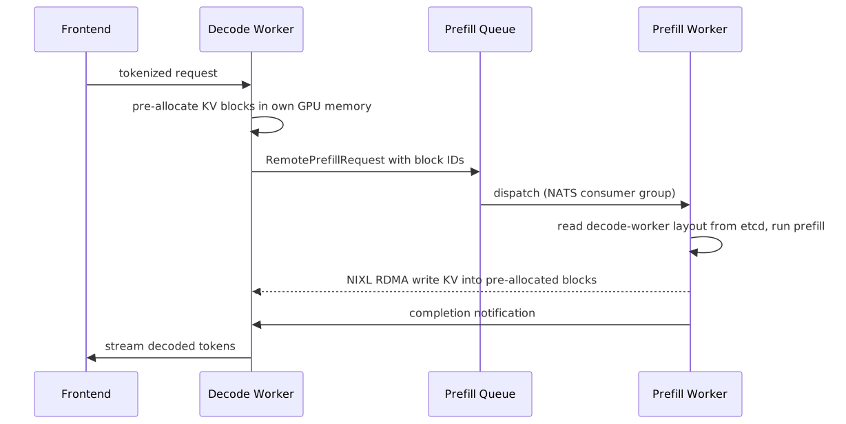
Two things fall out of that design. Because the decode worker pre-allocates the blocks before prefill starts, the memory layout is fixed in advance, so the NIXL transfer is a plain block copy to known addresses rather than a negotiation. And because every transfer is direct worker-to-worker, there is no centralized store left to bottleneck on, the failure mode that sank earlier prototypes. On top of that, Dynamo runs vLLM, SGLang, or TRT-LLM as the per-worker engine (through its make_engine interface), and a Planner scales the prefill and decode pools independently off Frontend metrics, which is the Kubernetes-native version of DistServe’s independent-scaling argument.
llm-d is a CNCF Sandbox project (accepted March 2026; v0.5.0) led by engineers from Red Hat, Google, IBM, and the vLLM and Kubernetes communities. It’s the Kubernetes-native disaggregated inference stack, and it maps the Dynamo architecture onto standard K8s primitives:
- xPyD architecture: X prefill workers and Y decode workers run as independent Kubernetes Deployments with separate HPAs (Horizontal Pod Autoscalers). The
x:yratio is a tunable. DeepSeek’s production ratio of 3:9 (prefill:decode, 3 prefill nodes and 9 decode nodes of 8 H100 each) is one data point, and our ratio depends on our prompt-length distribution. - Inference Gateway (IGW): built on the Gateway API Inference Extension, it handles KV-aware routing, directing follow-up requests to the Decode Worker that already holds the session’s KV cache and avoiding redundant transfers.
- NIXL transport: llm-d uses NIXL (the same library as Dynamo) for prefill-to-decode KV cache transfers, with support for both RDMA (InfiniBand or RoCE) and datacenter TCP fallback.
- Multi-tier prefix caching: L1 (GPU VRAM), L2 (CPU DRAM), and L3 (distributed, cross-worker). This extends vLLM’s APC to a fleet-wide cache, so prefix hits can occur even on a different physical worker than the one that originally computed them.
- Multi-accelerator support: the roadmap includes AMD (MI300X) and heterogeneous TP across GPU types, not just homogeneous NVIDIA clusters.
The practical difference is one of posture. llm-d is infrastructure-layer glue for teams already running Kubernetes, while Dynamo is NVIDIA’s opinionated full-stack solution. If we’re on EKS, GKE, or AKS and want to plug disaggregated serving into an existing GitOps pipeline, llm-d is the path. If we want NVIDIA’s turnkey stack with their support, Dynamo is the path. Both use NIXL underneath.
Beyond NVIDIA. This transport layer is no longer NVIDIA-only. In August 2026 Google open-sourced Raiden , the TPU-native counterpart to NIXL: the same job (chip-to-chip KV transfer for the prefill/decode handoff, cross-VM transfer over the network, and offloading KV blocks from TPU memory down to host DRAM), scoped to Google’s own DMA engines and inter-chip interconnect, and wired into both the JAX and PyTorch/XLA serving paths. It is early (Google marks it as not yet ready for general use), but its existence is the point: the prefill/decode handoff is becoming a cross-vendor commodity layer rather than a CUDA-only trick.
6. Outside CUDA: other accelerators
Everything up to here has quietly run on NVIDIA. The recipe, the day-zero kernels, the vLLM flags, even the bug: all of it was CUDA, because that is where DeepSeek V4 landed first and where vLLM ships kernels on release day. That is a bigger assumption than it looks, so it is worth double-clicking into that.
The ideas in this series can transfer fine to other hardware: the roofline, the memory-bound decode step, KV handoff, continuous batching are all just physics and none of them care who made the chip. What does not travel is the stack that implements them.
So the question this section actually asks is narrow and practical: when we step off NVIDIA silicon, how much of our serving stack comes with us? The short answer is that a thin top layer ports almost for free and a thick bottom layer does not, and Figure 13 draws where that line falls (as of this writing), not which box to buy:

What is outside the CUDA default:
- AMD ROCm is the most credible CUDA alternative for general GPU serving: HIP ports most kernels mechanically, Triton runs natively, and the MI300X’s 192 GB of HBM3 can win on memory-capacity-bound MoE serving. The gap is day-zero support: new architectures typically trail CUDA by days to weeks in vLLM/SGLang.
- Huawei Ascend (910C/950, CANN, the
vllm-ascendplugin) is the default inside China and is directionally competitive with Hopper-class inference on vendor benchmarks. Getting DeepSeek V4 Flash running on Ascend 910 has meant, per field reports piling up in the vllm-ascend issue tracker , on the order of a dozen source-level patches: turning off high-throughput EP features (including fused hash routers like the one from our bug), replacing CUDA-specific memory ops, and falling back to safer, slower paths. Roughly 60-70% of equivalent H200 throughput after patching is a fair ballpark from those write-ups, not a promise from a controlled bake-off. - Google TPUs are a different animal, not a drop-in GPU. The software path is XLA / JAX (and increasingly PyTorch/XLA), not vLLM-on-day-zero, but the serving stack is maturing fast: a vLLM TPU backend, JetStream, and, as of August 2026, an open-sourced KV-transfer layer ( Raiden , the TPU sibling of NIXL from section 5). Frontier labs use TPUs at scale; most open serving recipes above still assume GPUs. Worth knowing they exist, and that the tooling gap is closing, but still the wrong mental model to treat them as “another ROCm.”
- Inference ASICs are specialized silicon aimed at the decode bandwidth wall. Groq keeps weights in SRAM for dramatic batch-1 tokens/s. Cerebras is wafer-scale with a different capacity/latency story than Groq’s LPU pitch. Etched is transformer-specialized. Single-stream slides can look incredible; capacity and batch economics look different. Benchmark our own model.
Why this matters for the physics. The SRAM-resident designs are the cleanest test of the roofline from Part 1 , and they pass it. Decode is bandwidth-bound because every step streams the whole weight set out of HBM, so that ~42ms floor was never more than model-bytes divided by HBM bandwidth.
Groq and Cerebras go straight at the denominator of that ratio: they hold the weights in on-chip SRAM at effectively terabytes per second, paying in capacity (SRAM is tiny next to 141 GB of HBM) to buy a bandwidth regime HBM cannot reach. They don’t ride the decode wall down, they move the floor out from under it.
That is the key point: the roofline, the memory-bound decode step, and $B^{\star}$ are the invariants, while HBM is just the NVIDIA-shaped assumption bolted on top. Swap the memory substrate and the numbers move, but the equation we plug them into does not.
What actually ports today:
| Portable | Not portable |
|---|---|
| PyTorch high-level ops, ONNX exports | Hand-written CUDA C++ with inline PTX |
| Triton kernels (with caveats) | NVIDIA-only libraries (cuDNN, TensorRT, Transformer Engine) |
| Anything that bottoms out in PyTorch primitives | Hardcoded warp-size or Hopper/Blackwell intrinsics |
Portable ORMs and standard SQL travel; stored procedures and vendor intrinsics do not. The portable layer is real and thin.
CUDA’s stickiness is 15+ years of libraries and the reality that many new transformer architectures land on NVIDIA first. DeepSeek V4 had day-zero CUDA support; other stacks trail. That lag is the moat, and it is why the worked example here is a CUDA/vLLM story even when the concepts (roofline, KV handoff, continuous batching) apply elsewhere. It is worth noting the moat is being chipped away at one library at a time - for example Google open-sourcing Raiden to give TPUs a NIXL-equivalent, and NVIDIA itself opening its cuFile storage APIs; it would seem the serving substrate is slowly turning into cross-vendor plumbing.
7. Scheduling, queueing, and fleet-level routing
Continuous batching decides what happens on one GPU. Once we have a fleet, especially a disaggregated one, the same prefill/decode conflict becomes a queueing and routing problem: which request runs next, which worker gets it, and what we do when KV memory is full. This is the control plane sitting above every worker: the objectives we measure, and the failure modes those objectives create.
vLLM’s scheduler faces a multi-objective problem: maximize throughput, meet P99 TTFT, and meet TPOT. These fundamentally conflict and create tension with each other, with the batch size as the knob in the middle. Throughput wants big, full batches, because one weight load then serves as many tokens as possible. On the other hand, as we know a full batch is exactly what hurts the latency SLOs. And a new request is waiting behind everything already queued (worse TTFT), and every extra sequence sharing the step adds KV traffic to each decode (worse TPOT). Push the batch up for throughput and latency degrades; and if we hold it down to protect latency the throughput drops. 🙄
So the honest answer is that we do not solve this tension, we pick a point on it: the largest batch that still clears our latency SLO. Past that, the extra throughput lands on requests that already blew their deadline, which is worth nothing to the user. That SLO-bounded throughput is goodput, and it is what a real deployment tunes for rather than raw tokens/s. Watch the scan line in Figure 14 sweep the batch size up: throughput climbs, latency climbs, and goodput rides the throughput curve until latency hits the SLO, then falls off a cliff as requests start missing their deadline. The peak is the operating point.
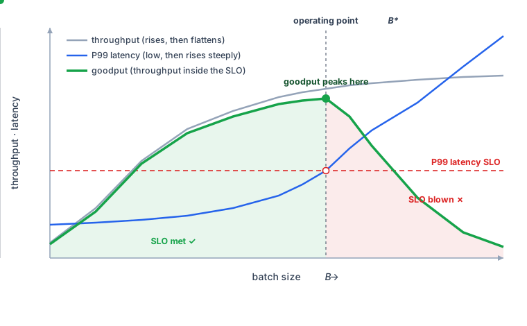
Let us walk through this from left to right, with batch size $B$ growing along the x-axis. Three curves are moving at once.
- The grey line is throughput: it climbs fast at small $B$ (each added request fills idle GPU) and then flattens, because once the batch is large enough the GPU is saturated and more requests buy almost nothing.
- The blue line is P99 latency: nearly flat while there is slack, then it knees upward hard, because a fuller batch means every request waits longer to be admitted (TTFT) and shares more KV traffic per step (TPOT).
- The dashed red line is our latency SLO, the promise we made to users. The one moment that matters is where blue crosses red: that vertical marker is the operating point $B^{\star}$, the largest batch we can run while still keeping the promise.
- The green line is goodput, and it is the whole point of the picture: to the left of $B^{\star}$ it tracks throughput upward (those tokens landed inside the SLO, so they count), but the instant latency crosses the SLO it falls off a cliff, because past that batch size the extra tokens are being delivered late and a late answer is worth nothing.
So the green curve peaks exactly under the crossing: raise $B$ short of that and we leave throughput on the table, push it past and we are just manufacturing SLO violations. Tuning a deployment is finding that peak and sitting on it.
7.1 Head-of-line blocking
Head-of-line blocking is when one long request at the front of a queue stalls many short ones behind it, even though the short ones would finish quickly on their own. Under FCFS (first-come-first-served), a single 10,000-token prompt can block 100 requests with 50-token prompts. The 100 short requests would each complete in seconds; instead, they wait much longer.
Whilst this might seem as a new class of issues and problems, it is worth highlighting that the same class of problem TCP solves with multiplexing, HTTP/2 with streams, and databases with connection pooling. Continuous batching removed intra-batch padding waste; fleet queues reintroduce HOL at the admission boundary.
The theoretical optimum for minimizing average response time is SRPT (Shortest Remaining Processing Time) - always run whichever request has the fewest tokens left to generate. The one catch though - we don’t know the LLM output length in advance, since requests don’t declare how long their generation will be.
ALISE (2024) addresses this with speculative scheduling, estimating the remaining generation length using embeddings from the model itself, predicting whether a request is “short” or “long” before it finishes, and using that prediction to set priority. This is analogous to predicting query cost before execution in a database query planner.
Figure 15 lines the two orderings up, the FCFS stall on top against the length-aware drain below:

7.2 Preemption and KV cache eviction
When GPU memory is full, and a higher-priority request arrives, we need a way to free capacity without dropping the whole queue. Preemption suspends a running request so another can run: its KV blocks are swapped to CPU or dropped, and the request resumes later (recompute or reload). Without it, admission becomes all-or-nothing and long sessions hog HBM forever.
Priority of the request here is assigned, not discovered as the model has no notion of it. Usually it comes from an explicit priority field on the request, a tier or SLA class (paid versus free, interactive versus batch), or a deadline signal that a request is close to missing its SLO.
vLLM supports this OOB, though only under its opt-in priority scheduling policy; the default is FCFS, where the sole ordering is arrival time and preemption just frees KV from the most recently admitted requests. If a high-priority request arrives and the GPU is full, a low-priority running request can be suspended: its KV cache blocks are evicted to CPU memory or dropped, and it’s resumed later by recomputing its KV cache. The cost of recomputing is proportional to the prompt length already processed, and the cost of swapping is proportional to the KV cache size. For long-context requests, swapping is cheaper; for short ones, recomputing is cheaper. vLLM tracks this and chooses dynamically.
At scale, across a fleet of prefill and decode workers in a disaggregated setup, the scheduling problem becomes a routing problem. The router must balance prefill-worker utilization, decode-worker KV cache capacity, inter-worker network bandwidth, and request SLO deadlines. This is an active research area, and most production systems use heuristics (weighted round-robin, least-loaded) rather than optimal schedulers, because the optimal scheduler requires output-length prediction that’s not yet reliable enough.
7.3 Measuring the objectives
None of these objectives mean anything without a way to measure them, and the numbers above (TTFT, TPOT, throughput) come from a specific kind of experiment. The standard practice is to run a load generator that replays a realistic distribution of prompt and output lengths while sweeping the request arrival rate, and to record four things at each rate: TTFT (usually P50 and P99), TPOT or inter-token latency, end-to-end throughput in tokens per second, and goodput. This throughput counts only requests which stayed inside their SLO.
Goodput is the one that matters, because raw throughput keeps climbing right up until latency collapses, and only goodput captures the point where the system quietly stops meeting its promises.
Here “sweep” just means we run the benchmark repeatedly rather than once, nudging the request rate up a rung each time and recording the four metrics at every step. vLLM ships exactly this as a first-class tool. vllm bench serve (the successor to the older benchmark_serving.py) drives load against a running server at one chosen rate, and the load-bearing flag is --goodput, which takes the SLO thresholds directly, so goodput stops being a metric we compute by hand and becomes one the harness reports:
# one point on the sweep: 12 requests/s against a live server,
# with the SLO stated as TTFT P99 ≤ 2000ms and TPOT P99 ≤ 50ms
vllm bench serve \
  --model deepseek-ai/DeepSeek-V4-Pro \
  --dataset-name sharegpt \
  --dataset-path ShareGPT_V3_unfiltered_cleaned_split.json \
  --request-rate 12 \
  --num-prompts 1000 \
  --percentile-metrics ttft,tpot,itl,e2el \
  --goodput ttft:2000 tpot:50
That command is one rung. Run it across the whole ladder (--request-rate 2, 4, 8, 12, 16, 20, then inf for the saturation point) and read the reported P99s and goodput off each run. Laid out, the numbers trace the exact shape Figure 14 draws, only now against arrival rate rather than batch size:
| Arrival rate (req/s) | P99 TTFT (ms) | P99 TPOT (ms) | Output tok/s | Goodput (req/s) |
|---|---|---|---|---|
| 2 | 180 | 22 | 1,900 | 2.0 |
| 4 | 240 | 28 | 3,700 | 4.0 |
| 8 | 520 | 41 | 7,000 | 8.0 |
| 12 | 1,400 | 58 | 9,100 | 9.4 |
| 16 | 3,900 | 96 | 9,600 | 4.1 |
| 20 | 8,800 | 150 | 9,700 | 1.0 |
The last two columns are the whole story.
- Output tok/s keeps climbing all the way to saturation, and if that were our headline number we would happily run at 20 req/s. *
- Goodput tells the truth: it tracks the arrival rate up to about 12 req/s, then at 16 the TPOT P99 has blown past the 50ms SLO and most requests no longer count, so goodput collapses even though the GPU is busier than ever.
- Operating point: It is that turning point between rows 12 and 16, where goodput stops climbing and rolls over: the same $B^{\star}$ crossing from Figure 14, now expressed as the maximum arrival rate the deployment can sustain inside its SLO.
A few practices keep these numbers honest. Skip any one of them and the goodput figure quietly lies (it is still a throughput number, and seems more like a watermelon effect than a real SLO):
- Replay a realistic trace, not uniform load. That turning point moves with the prompt and output length mix, so a ShareGPT-style distribution (or our own logged traffic) measures our system; fixed-length synthetic prompts measure a fiction.
- Report P99, not the mean. The SLO governs the tail, and a healthy mean routinely hides a P99 that is already violating it.
- Fix the SLO before comparing. Goodput is undefined without stated TTFT and TPOT thresholds; two engines or parallelism layouts only compare at the same SLO.
- Decide cold versus warm on purpose. A pre-warmed prefix cache (APC) inflates goodput against a cold start, so pick the one that matches production and hold it constant across runs.
- Pin everything. Engine version, flags, quantization, and batching regime all move these curves, for the same reason the determinism section gave: the measurement is only as reproducible as the stack under it.
That is the right way to compare an engine, a parallelism layout, or a chunk-size setting: fix the SLO, step the arrival rate up, and find the point where goodput peaks before it rolls over.
8. How agentic workloads stress the stack
Everything so far has been machinery, the levers that make a single request economical. What is left is the traffic that drives it, and two request shapes lean on the stack hardest: agents and reasoning. An agent loop breaks the clean prefill-then-decode shape of a chat request: it interleaves bursts of tool-result prefill with stretches of quiet decode, and the KV cache keeps growing turn after turn because it is all one long session.
Yikes. The scheduler has to juggle that bursty traffic, and the KV cache has to hold it all, or the whole thing collapses. 😊
8.1 KV grows every turn
A multi-turn agent session accumulates KV cache across many rounds of user message, model response, tool call, tool result, model response, and so on. Each tool call adds tokens to the context, and each tool result can add a great many tokens. The decode memory-bandwidth bottleneck gets steadily worse as the session grows, because every new token now streams a larger KV cache out of HBM.
Put numbers on it with the ~320 KB/token GQA figure from prefix caching . It is not uncommon for a coding agent to open on a 2K-token system-plus-task prompt, then add another ~2K tokens of tool result per round. After ten rounds the context is north of 20K tokens, so its KV cache alone is $20\text{K} \times 320\text{ KB} \approx 6.4$ GB for that one session, and it only grew there.
Needless to say this is a double whammy - one it holds up the HBM that could have served other requests, and two it drags decode down, because the KV-traffic term $B \cdot L \cdot m_{\text{KV/token}}$ from Part 1 scales with context length $L$. The same model that decodes a fresh chat quickly decodes turn ten of an agent loop slower, token for token, because each step is streaming ten times the KV. MLA or a linear-attention hybrid (section 2.4) would turn that 6.4 GB into a small fraction of it.
8.2 The re-prefill problem, and why prefix caching carries agents
The re-prefill problem is where an agent loop hurts most, and it is the part the user actually feels. When a tool returns a result, e.g. 2K-token JSON blob from a web search, that result has to be processed as a new prefill event mid-session, and TTFT spikes every time. From the user’s side this is the “thinking pause” between the agent deciding to call a tool and it answering. Chunked prefill (section 1.4) is the direct mitigation, because a tool-result prefill is exactly the bursty, large-prompt event that chunked scheduling was built to smooth.
But the lever that actually makes agents affordable is prefix caching. The naive reading of the loop is alarming: if the context grows to 20K tokens, do we re-prefill all 20K every turn? That would be quadratic in the number of turns and would sink the workload on its own. We do not, because everything except the newest tool result is a prefix the engine has already seen. With Automatic Prefix Caching the stable history is already resident in the KV cache, so a tool round-trip pays prefill only for the new blob, not the whole conversation. The catch is that the cache has to still be there: this only helps if the session lands back on a worker that holds its blocks, which is precisely the per-session KV affinity that LMCache and Mooncake add on top of disaggregation. If we were to lose that affinity then every turn re-prefills from scratch, and we are back to square one, with the quadratic cost coming back.
8.3 When the session outgrows the cache
Prefix caching keeps the per-turn cost flat, but nothing stops the total context from growing until it hits a wall. An agent that runs long enough fills its share of KV memory, and then something has to give. There are three ways to make room, and they differ in who does the work, the engine or the application:
- Evict and recompute (the engine handles it). When the GPU runs out of KV memory, the scheduler suspends the session, moves its KV blocks out to CPU memory or throws them away entirely (the preemption mechanism from section 7.2), and then re-prefills the context when the session gets its turn again. This needs no cooperation from the application, which is why it is the default fallback. The downside is that it undoes the very thing we just relied on: the prefix cache we were counting on to keep re-prefill cheap is exactly what gets discarded, so the session pays full prefill again when it resumes.
- Compact the history (the application handles it). Instead of holding the entire transcript, the application actively prunes it, dropping turns that no longer matter (a plan that was later revised, tool output that has been superseded) or replacing a long stretch of history with a short summary. This keeps the context small enough that KV never blows up in the first place. The catch is that the model now sees a different, shorter conversation than actually happened, so it is a product decision about what the agent is allowed to forget, not a knob the serving engine can turn on its own.
- Change the attention math (the architecture handles it). The linear-attention hybrids from section 2.4 sidestep the whole problem: instead of a KV cache that grows one entry per token, they fold the entire past into a fixed-size recurrent state that stays the same size no matter how long the session runs. A long agent session then stops paying more for its own length, because there is no growing cache to pay for. This is the cleanest fix, and it is why those architectures tend to show up first in agent-heavy and long-context products, but it requires choosing such a model up front rather than something we can bolt onto an existing deployment.
8.4 Fleets of agents
Everything so far has followed one agent session. Run a fleet of them and a new problem appears that no single session shows: the load stops being smooth. A chat fleet is a crowd of roughly interchangeable requests, each a short prefill then a steady decode, so the aggregate arrival rate is what the scheduler from section 7 plans around.
An agent fleet is nothing like that. Each session lurches between a heavy tool-result prefill, a stretch of quiet decode, and a dead stop while it waits on an external tool, and those phases land out of step across sessions. At any one instant some agents are prefilling a fresh 2K-token blob, some are mid-decode, and some are blocked on a web call doing no compute at all.
The saving grace is that this unevenness partly averages out. Because the sessions are out of phase, the bursts overlap rather than stack: while one agent is mid tool-result prefill, a dozen others are quietly decoding, so the same continuous batching that fills a chat batch keeps the GPU busy here too, just with a lumpier arrival pattern. The scheduler is still juggling the identical prefill/decode mix from section 7, only now the two phases belong to different sessions of the same conversation rather than to unrelated requests, and each session carries the growing KV cache from section 8.1 with it the whole time.
That standing KV is what makes an agent fleet expensive in a way a chat fleet is not, and it shows up worst during the tool wait. An agent blocked on a slow tool call is generating nothing, but its context (2K, 20K, etc.) is still sitting in HBM, holding blocks that a runnable request could use. This is the fleet-level version of the outgrows-the-cache problem from 8.3: the engine can evict that idle session to CPU and pay to re-prefill or reload it when the tool returns, or it can let it squat on HBM and shrink the batch everyone else runs in. Of course, neither option is free, and the right call depends on how long tools typically block and how tight KV pressure is, which is why production agent stacks tune eviction against measured tool latency rather than leaving it to the default.
As it happens, disaggregation fits this shape quite well, because the two hard phases want opposite hardware. The bursty tool-result ingestion is compute-bound prefill, exactly what a prefill pool is provisioned for, so those spikes land on machines built to absorb them instead of stalling a decode. The long quiet inter-step reasoning is bandwidth-bound decode, which the decode pool streams.
And KV affinity, the same per-session pinning that LMCache and Mooncake add on top of disaggregation, becomes non-negotiable rather than a nice-to-have: an agent that comes back from a tool call has to land on the worker still holding its history, or it re-prefills the whole conversation and we are back to the quadratic cost 8.2 warned about. A router that scatters an agent’s turns across workers turns prefix caching off by accident.
Batch RL rollouts (the training-time mirror image). There is one agent workload where all of this inverts, and it is worth naming because it is where a lot of GPU time actually goes. When we generate rollouts for RLHF, GRPO, or PPO, thousands of agent trajectories run in parallel to produce training data, and there is no user waiting on any of them, so there is no latency SLO at all. Every trade we just made to protect the thinking pause inverts: we no longer care about TTFT or per-session TPOT, only about total tokens per GPU-hour, so the scheduler is free to run the largest, most compute-efficient batches it can and let any individual trajectory wait. That is the regime DAS (section 4.4) was built for, stretching or shrinking the draft length to match the non-uniform token distributions a rollout batch throws off. Same agent shape, inverted objective: interactive agents optimize the thinking pause a human feels, training rollouts optimize the tokens per GPU-hour that feed the next model.
8.5 What is off the shelf, and what stays our problem
It is easy to read the last four subsections as a pile of infrastructure we each have to build. Mostly, we do not. Almost every mechanism named above already ships in vLLM or a library next to it, and only a short list of product decisions is genuinely left to us, the ones the engine will not make on our behalf.
The growing KV cache from 8.1 is a solved problem in the sense that every lever against it is a flag or a library. Prefix caching is --enable-prefix-caching; KV quantization is --kv-cache-dtype fp8; the MLA and linear-attention shrinks are a model choice we make when we pick the checkpoint. When the session simply will not fit in HBM, LMCache tiers it out of GPU memory into CPU, local SSD, and remote stores (Redis/Valkey, Mooncake, S3, anything behind NIXL), so the cache spills instead of getting thrown away. Its published multi-turn and agentic benchmarks are this exact workload, not a hypothetical.
The re-prefill problem from 8.2 is the strongest off-the-shelf story of the lot. Automatic Prefix Caching (vLLM) and RadixAttention (SGLang) already skip the stable history; LMCache goes one step past naive prefix caching with CacheBlend, which reuses cached KV blocks that sit in the middle of a prompt rather than only at the shared head, recomputing just enough tokens to keep quality. The per-session affinity that 8.2 said we cannot lose is not something we hand-roll either, it comes from the KV-aware routers below.
The fleet routing and disaggregation from 8.4 have more than one production-grade home. The vLLM production-stack router does session-ID and KV-cache-aware placement; AIBrix adds a distributed cross-engine KV cache and even ships an agent-session workload generator to benchmark against; llm-d and NVIDIA Dynamo carry KV-aware gateways over NIXL/RDMA; the SGLang router does cache-aware load balancing. Any one of them gives us the affinity and the prefill/decode split without writing a scheduler. And the RL-rollout corner is a framework decision, not an engine we build: veRL, OpenRLHF, slime, and AReaL all drive vLLM or SGLang as their generation backend, with DAS as the algorithm riding on top.
That leaves a short list of things no library will decide for us, and it is worth being honest that this is where the real work is:
| Concern | Off the shelf | Stays our problem |
|---|---|---|
| KV growth (8.1) | APC, FP8 KV, MLA/linear models, LMCache tiering | Which checkpoint and cache budget to pick |
| Re-prefill (8.2) | APC, RadixAttention, LMCache + CacheBlend | Nothing much, this one is basically solved |
| Session outgrows cache (8.3) | Engine eviction/swap, token-level KV compression (StreamingLLM, H2O, SnapKV, R-KV) | History compaction: what the agent is allowed to forget |
| Fleet routing (8.4) | production-stack, AIBrix, llm-d, Dynamo, SGLang router | Tool-wait eviction policy tuned to our tool latency |
| RL rollouts (8.4) | veRL, OpenRLHF, slime, AReaL + DAS | Reward shaping and trajectory design, not serving |
The two bold cells are the key points. Token-level KV compression can decide which cached tokens to drop, but it cannot decide that a superseded plan or a stale tool result is semantically safe to summarize away; that is application logic about our agent’s task, and it changes what the model sees, so the engine correctly leaves it to us.
Likewise, every router exposes the mechanism to evict an idle session during a tool wait, but the policy, evict aggressively versus let it squat, only makes sense against our own measured tool-call latencies.
There is a catch here that gets worse as the fleet grows. Pulling a block off the shelf gives us the component, not the system. On a single node most of these are genuinely drop-in. Across thousands of accelerators, often a mix of NVIDIA, AMD, and Ascend or TPU, the work shifts to making the blocks agree with one another. The KV-aware router needs a live view of cache residency that matches what the LMCache tier and the disaggregation planner actually hold, or it sends a session to a worker that evicted its blocks a second ago. The autoscaler has to add and drain prefill and decode pods without stranding a session mid-tool-call. Prefix hits have to survive the rolling image upgrade that is always touching some slice of the fleet. And each of those coordination points has to hold across vendors whose KV layouts, transport libraries, and day-zero support do not line up, which is what section 6 was really about. None of it is a missing algorithm. It is integration, capacity planning, and operations, the work a single --flag quietly hides. The blocks are commodity; wiring them into one coherent fleet is still ours, and it gets harder as the accelerator count climbs and the silicon stops being uniform.
9. Inference-time scaling: spending tokens to buy quality
As we saw, agents change the shape of traffic; on the other hand inference-time scaling changes the amount, and it is the shape that has grown fastest. Everything above optimized for cheaper tokens. This dial buys more tokens for better answers without retraining (o1/o3-class, DeepSeek R1, Gemini thinking, and the reasoning effort knobs). Model-side depth is in the reasoning models post ; here we only care what it does to the compute/bandwidth balance and the fleet.
9.1 Reasoning effort is a dial on decode
A classical chat request is short prefill, and short-to-medium decode. A reasoning request is short prefill, then a long hidden decode of thinking tokens (often wrapped in <think>…</think> or an equivalent internal channel), then a shorter visible answer. That middle stretch dominates the user-facing latency. Some vendors have started exposing it as an explicit knob rather than a prompt hack: OpenAI-style reasoning effort (low / medium / high, sometimes with a token budget), Qwen’s thinking-token cap, NVIDIA NIM’s thinking budget, and similar controls that say “spend up to $N$ tokens thinking before you answer.” Figure 16 draws the timelines:
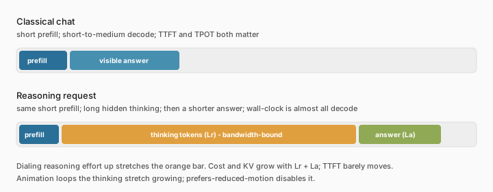
The reasoning-effort knob is not cosmetic. Raising effort moves us deeper into the memory-bandwidth-bound regime for longer. Each thinking token still has to stream the model weights (or the active MoE experts) from HBM. Horace He’s Making Deep Learning Go Brrrr framing still applies: if we’re bandwidth-bound, more FLOPs on the datasheet don’t help until we move less data or reuse what we loaded. Reasoning effort is the product decision that chooses how much of that bandwidth-bound work to buy per request.
We can put a number on this cost with the formulas we already have, nothing new. Raising effort spends two resources, and there is one equation for each: the wall-clock time decode runs, and the KV memory it has to hold. Writing $L_p$ for the prompt, $L_r$ for the thinking tokens, and $L_a$ for the answer, and reusing $T_{\text{mem}}(B)$ and $m_{\text{KV/token}}$ from earlier:
$$ T_{\text{decode}} \propto (L_r + L_a) \cdot T_{\text{mem}}(B), \qquad M_{\text{KV}} \propto (L_p + L_r + L_a) \cdot m_{\text{KV/token}} $$
The left equation is time: every token after the prompt pays one bandwidth-bound decode step, so decode runs almost linearly longer as the thinking budget grows.
The right is memory: every token that ever entered the cache keeps costing KV, and a thinking token counts the same as an answer token, so a long <think> block can dominate HBM even when the visible answer is short. These are the two we track because they are the two the effort knob actually moves, and $L_r$ sits inside both.
Put the ~320 KB/token GQA figure against a few budgets and the cost is concrete:
| Reasoning budget $L_r$ | Extra KV $\approx L_r \cdot 320$ KB | Relative decode work vs $L_r{=}2$K |
|---|---|---|
| 2K (low) | ~0.6 GB | 1× |
| 4K (medium) | ~1.3 GB | ~2× |
| 8K (high) | ~2.6 GB | ~4× |
| Best-of-$k$ at 4K | ~$1.3 \times k$ GB | ~$2k\times$ vs single 2K |
An 8K high-effort trace is already a ~2.6 GB KV slab for one request before the base weights, and best-of-$k$ multiplies both columns by $k$ since we run $k$ independent traces. Accuracy usually improves much less than linearly with $L_r$, which is why every serious deployment ends up sweeping the budget and picking a knee rather than always running “high.”
9.2 What changes in the stack
The short version is that a reasoning model turns a short request into a very long decode stream, and that hits every SLO and every layer above.
- TTFT stops being the headline metric. If the model is going to think for thirty seconds, nobody cares whether the first token lands in 40ms or 400ms. What matters is reasoning tokens per second (and time-to-final-answer), which is pure decode. This is where the decode-side levers earn their keep: speculative decoding, MTP, and quantization pay off more here than on any other traffic shape.
- KV cache pressure becomes the capacity limit. An 8K thinking trace is an 8K decode stream with a correspondingly large KV cache, on top of the prompt. Best-of-N and majority voting, where we sample $k$ candidate chains and keep the best, multiply that pressure by $k$ outright. Prefix caching helps the shared system prompt; it does almost nothing for the unique thinking tokens.
- Batching economics flip. Interactive chat wants moderate batch sizes to protect TPOT. Reasoning fleets often run fewer concurrent high-effort requests because each one already occupies a large KV slab for a long time. The continuous-batching machinery still applies, but the “good” operating point moves: we may never want batch sizes that push toward compute-bound if each request’s KV already fills the GPU.
- Reasoning effort becomes a scheduler input. Low-effort and high-effort requests are different animals. A naive FCFS queue lets one high-effort job block a pile of low-effort ones (head-of-line blocking again, but now the “length” is the thinking budget, not the prompt). Production systems increasingly need effort-aware admission control: separate lanes, priority by remaining budget, or hard caps per tenant.
- Verification is often a second model. Process reward models that score reasoning steps are themselves models being served alongside the generator: two model families, different batch shapes, sharing a cluster. That is like a mini-disaggregation problem, and it interacts with effort because higher effort produces more steps to score.
- Disaggregation still helps, but differently. Prefill workers stay lightly loaded on reasoning traffic (prompts are short). Decode workers become the scarce pool. Even a decode-heavy split like DeepSeek’s 3:9 prefill:decode from section 5.2 still assumes prompts long enough to keep the prefill pool busy; reasoning traffic breaks that assumption, so we skew harder still toward decode, and we care about KV affinity so a multi-turn reasoning session doesn’t re-prefill its growing trace.
9.3 Adaptive effort, not just more tokens
The research result that matters is that blindly maxing effort is wasteful. Snell et al. ( Scaling LLM Test-Time Compute Optimally ) and follow-on work show that easy problems want little or no extra thinking, medium problems want a modest budget (or a few parallel samples), and hard problems want deeper search up to a knee beyond which returns collapse.
In FLOPs-matched comparisons they report that, on some hard prompts, a smaller model with well-allocated test-time compute can match a model on the order of 14× larger that answers greedily. That is the same “don’t pay for FLOPs we can’t use” instinct as the roofline, now on the effort dial. Figure 17 is the compute-optimal picture:

In practice that means:
- Expose and log the budget. Treat thinking tokens like memory or p95 latency: a first-class metric per request, per tenant, per model.
- Default low, escalate on failure. Start with low/medium effort; retry or continue with a higher budget only when a verifier or confidence signal says the answer is weak.
- Separate interactive from batch. User-facing chat rarely wants “high” on every turn. Offline eval, agent planning, and math workloads do. Same weights, different serving pools, different effort defaults.
- Watch the hidden tokens. If our API bills or rate-limits only on visible output, high-effort traffic will surprise us on GPU-hours and on the bill. Count $L_r$ explicitly.
None of this changes the layers of the stack; it changes which ones we lean on, and it adds a product knob that maps almost one-to-one onto decode bandwidth. Efficiency work (kernels, quantization, speculative decoding, disaggregation) buys cheaper tokens. Reasoning effort decides how many of those tokens a request is allowed to burn. A serving stack tuned for interactive chat will look very different from one tuned for high-effort reasoning rollouts, even when the model weights are identical.
🎉 If you have read this far in one pass, your context window is genuinely impressive, no KV eviction, no summarization, full attention over a very long document. That is more than most models manage without spilling to CPU. So go recompute yourself: drink some water (you are more bandwidth-bound than you think), stretch the meat-based actuators, refill your token budget, and maybe pet a GPU if one is nearby. The bug will still be fixed when you get back. 🚶
Part 3 recap: serving at scale is Parts 1
and 2
composed under a real traffic shape. The serving engine turns the request path into a scheduler, a paged KV cache, and an API; quantization, GQA, and MLA shrink the bytes each token moves; multi-LoRA and prefix caching stretch one GPU across more useful work; disaggregation stops a compute-bound prefill from stealing a bandwidth-bound decode’s SLO; and speculative decoding and MTP buy several tokens per weight load. Above all of it, the scheduler decides which request runs where when KV memory runs out, and none of it is CUDA-only anymore: the same levers reappear on ROCm, Ascend, and TPU with different names. Agents and reasoning models add no new physics; they only lengthen how far each request sits on the memory-bandwidth side of the crossover, which is why the decode-side levers matter most for them. Almost every one of these blocks now ships in vLLM or a library beside it, so the work left is less inventing them than wiring them into one coherent fleet. Read a recipe like DP+EP + FP8 KV + chunked prefill as exactly that: a set of choices about bytes, launches, and which pool runs which phase, tuned to the traffic we actually serve.
10. Revisiting the bug, layer by layer
With the layers in place, the opening incident is quick to re-read.
Root cause. Fused MoE router torch.ops._moe_C.topk_softplus_sqrt: DeepEP produced topk_indices as int64 while hash metadata could stay int32. The CUDA dispatcher inferred pointer widths from topk_indices, so int32 tensors were read as int64. Crash at profile_run, before any token.
Why each escape hatch failed (now readable as layer facts):
| Escape hatch | Why it didn’t help |
|---|---|
--enforce-eager | Turns off Graphs / compile (Part 2). The dtype mismatch is inside the C++ op. |
Disabling torch.compile | Inductor treats torch.ops._moe_C.* as opaque. Schema visible; kernel internals not. |
Blanket cast to int64 | token_expert_indices must stay int32. No single dtype fits every slot. |
TP=8 fallback | Different MoE path; never enters the fused DP+EP hash router. Slower, but alive. |
The fix (
#43425
, merged 2026-06-11, 01e7bebf34b4
): in vllm/_custom_ops.py, align input_tokens and hash_indices_table to topk_indices.dtype before launch; leave token_expert_indices as int32. One selective cast, invisible above the kernel. The report I filed, issue #40862
, was closed the same day the fix landed; the dtype fix itself is #43425, while DeepEP v2 (#41183)
is the broader MoE expert-parallel rework that maintainers flagged as the longer-term home for this path, not the root-cause fix.
Same class of bug as ORM types into a C extension with a stricter contract. Fix the extension, not the app.
Catching it before production is three ordinary engineering moves. (1) Test dtype contracts on custom ops across caller combinations (the regression the fix added). (2) Smoke the pinned image in CI with the same profile_run path that crashed; treat image tag + parallelism config as a deployable event. (3) Pin and verify rolling tags: record the vLLM commit with our flags. We don’t need to understand fused MoE routers to catch this. Smoke the pinned image, and treat the serving stack as the production dependency it is.
Filed, fixed, shipping.
11. Takeaways
Three parts, three takeaways.
Part 1 · every request is two workloads. Prefill sets TTFT (compute). Decode sets TPOT (bandwidth). Near ~300 FLOPs/byte is the crossover. Its phase-and-lever figures are the useful mental model: put each technique under prefill, decode, or handoff.
Part 2
· abstractions leak at the kernel boundary. Graphs and torch.compile optimize launch sequences; they do not rewrite C++ op contracts. That is why the opening knobs failed and why FlexAttention matters as the exception that dissolves one important boundary.
Part 3 (this post) · recipes are compositions of Parts 1 and 2 under a traffic shape. DP+EP, FP8 KV, chunked prefill, disagg, speculative decoding, multi-LoRA, effort knobs: each is a lever on bytes, launches, or which pool does which phase. Agents and reasoning fleets do not invent new physics; they change how long we sit on which side of the compute/bandwidth crossover. Figure 18 is the stack in one picture:

LoRA fleets and agent loops don’t invent new physics. They still come down to bytes moved, kernels launched, KV handed off, and dtype contracts nothing above the C++ line can see.
The bug is fixed. The layers aren’t. 😏
Related reading: Modular’s LLM Inference Handbook
is the complementary reference, a broad non-linear lookup across deployment and ops. This series goes the other way: one continuous derivation down the stack, from vllm serve to the kernel, anchored to a single bug. It has no roofline derivation, compilation pipeline, or kernel forensics, which is exactly the half we get across Part 1
, Part 2
, and this post.
Series wrap-up
That is the whole stack, from the physics of one request down to the kernel and back up to a fleet. The three parts compose into one mental model:
- Part 1 · Physics of a request : every request is two workloads. Prefill is compute-bound (sets TTFT); decode is bandwidth-bound (sets TPOT). The crossover near ~300 FLOPs/byte and the batch target $B^{\star}$ are why batching exists.
- Part 2 · Below Python
: abstractions leak at the kernel boundary. CUDA Graphs and
torch.compileoptimize launch sequences; they do not rewrite the C++ dtype contracts inside a kernel. That is why the opening knobs failed. - Part 3 · Serving at scale (this post): recipes are compositions of Parts 1 and 2 under a traffic shape. Every lever pulls on bytes moved, kernels launched, or which pool runs which phase.
The bug is fixed. The layers aren’t, and now we can read them.
- ← Part 1 · Physics of a request
- ← Part 2 · Below Python
- Part 3 (this post) · Serving at scale
References & Further Reading
Grouped by topic; starred (★) entries are the best starting points. These cover Part 3; Parts 1 and 2 carry their own reference blocks.
vLLM and serving systems
- ★ Efficient Memory Management for Large Language Model Serving with PagedAttention (Kwon et al., SOSP 2023)
- vLLM official documentation
- vLLM Large Scale Serving: DeepSeek @ 2.2k tok/s/H200 with Wide-EP (vLLM blog)
- SGLang: Efficient Execution of Structured Language Model Programs (Zheng et al., NeurIPS 2024) (RadixAttention / prefix caching)
- SGLang documentation
- NVIDIA TensorRT-LLM (GitHub)
- Hugging Face Text Generation Inference (TGI)
- LMDeploy (InternLM / SenseTime)
- llama.cpp / Ollama (local and edge serving)
- XGrammar: Flexible and Efficient Structured Generation Engine for LLMs (Dong et al., MLSys 2025) (constrained decoding backend)
Quantization
- AWQ: Activation-aware Weight Quantization for LLM Compression and Acceleration (Lin et al., MLSys 2024)
- GPTQ: Accurate Post-Training Quantization for Generative Pre-trained Transformers (Frantar et al., ICLR 2023)
- FP8 Formats for Deep Learning (NVIDIA / Arm / Intel)
- NVIDIA Transformer Engine documentation
- DeepSeek-V3 Technical Report (DeepSeek-AI, 2024) (native FP8 training/serving at scale)
- GQA: Training Generalized Multi-Query Transformer Models from Multi-Head Checkpoints (Ainslie et al., EMNLP 2023)
- DeepSeek-V2: A Strong, Economical, and Efficient Mixture-of-Experts Language Model (DeepSeek-AI, 2024) (introduces Multi-Head Latent Attention)
- ★ The Inference Engineering Masterclass (Philip Kiely and Ali Taha, Baseten × Latent Space, 2026) (source for NVFP4 as a Blackwell-native path, and the layer-selection result validated with a distributional perplexity check rather than benchmark scores)
Multi-LoRA serving
- ★ LLM Customization and Fine-Tuning: Adaptation, Distillation, and Alignment (Bahree and Tok, Manning MEAP, 2026) (building the fine-tunes this section serves: LoRA/QLoRA, SFT, distillation, and DPO, end to end on a single GPU)
- S-LoRA: Serving Thousands of Concurrent LoRA Adapters (Sheng et al., MLSys 2024)
- Punica: Multi-Tenant LoRA Serving (Chen et al., MLSys 2024)
Speculative decoding
- ★ Fast Inference from Transformers via Speculative Decoding (Leviathan, Kalman, Matias, Google, ICML 2023)
- ★ Looking back at speculative decoding (Google Research) (source of the speculative-decoding animation earlier in the post)
- Accelerating Large Language Model Decoding with Speculative Sampling (Chen et al., DeepMind, 2023)
- Medusa: Simple LLM Inference Acceleration Framework with Multiple Decoding Heads (Cai et al., ICML 2024)
- EAGLE: Speculative Sampling Requires Rethinking Feature Uncertainty (Li et al., ICML 2024)
- Better & Faster Large Language Models via Multi-token Prediction (Gloeckle et al., ICML 2024) (the training-time idea behind DeepSeek’s MTP)
- Qwen3.8-2.4T-A95B (Qwen Team, 2026) (open Qwen-Max-class MoE, 2.4T total / 95B active, trained with multi-step MTP; the earlier Qwen3-Next introduced MTP to the Qwen line)
- Qwen3.8-27B (Qwen Team, 2026) (MTP in a compact dense vision-language model, trained with multi-step MTP; served by vLLM, SGLang, and TokenSpeed)
- DSpark: Confidence-Scheduled Speculative Decoding with Semi-Autoregressive Generation (DeepSeek-AI, 2026) (semi-autoregressive drafting plus load-aware verification scheduling; replaced the MTP-1 baseline in DeepSeek-V4 production)
- GLM-4.5: Agentic, Reasoning, and Coding (ARC) Foundation Models (GLM-4.5 Team, 2025) (ships an MTP layer used as an EAGLE-style speculative head; covers GLM-4.5 and GLM-4.6)
- GLM-5: from Vibe Coding to Agentic Engineering (GLM-5 Team, 2026) (GLM-5.2 flagship, 753B MoE; improved MTP head for speculative decoding, up to 20% higher acceptance length, and the IndexShare sparse-attention scheme)
- ★ Speculative Decoding: Getting K Tokens for the Price of One (Salman Quazi)
- Inference Engineering (Philip Kiely, Baseten) (traffic-specific speculators on dedicated deployments, and the stacked-optimization path to ~10×)
- Together AI Research (DAS, Kitty, ThunderKittens, ParallelKittens)
MoE and Expert Parallelism
- DeepEP: Open-source MoE all-to-all communication library
- An introduction to Mixture of Experts (Bahree, Desigeek)
- Mixture of Experts Explained (Hugging Face)
Disaggregated serving (production frameworks)
- NVIDIA Dynamo documentation
- NVIDIA Dynamo architecture flow (NIXL transfer protocol, etcd coordination, NATS prefill queue)
- NIXL: NVIDIA Interchange Library (GitHub) (block-based GPU-to-GPU transfer abstraction)
- LMCache: KV cache offloading and sharing
- llm-d: Kubernetes-native disaggregated inference stack, xPyD and multi-tier prefix caching (CNCF Sandbox)
The multi-vendor landscape
- AMD ROCm documentation
- SemiAnalysis: MI300X vs H100 vs H200 inference benchmarks
- Groq: LPU inference architecture overview
- vllm-ascend: Huawei Ascend NPU support for vLLM
- TPU Raiden: Google’s open-source TPU KV-cache transfer library (the NIXL analog for TPUs)
Agentic AI and inference
- The Hitchhiker’s Guide to Agentic AI (arXiv:2606.24937)
- vLLM production-stack: K8s-native reference serving with a session-ID and KV-cache-aware router
- AIBrix: cost-efficient GenAI inference infrastructure with a distributed cross-engine KV cache and an agent-session workload generator (ByteDance) ( white paper, arXiv:2504.03648 )
RL rollout frameworks (the training-time side of agents)
- veRL / HybridFlow: A Flexible and Efficient RLHF Framework (Sheng et al., arXiv:2409.19256)
- OpenRLHF: An Easy-to-use, Scalable and High-performance RLHF Framework (Hu et al., arXiv:2405.11143)
- slime: an SGLang-native post-training framework for RL scaling (THUDM)
- AReaL: A Large-Scale Asynchronous Reinforcement Learning System (Fu et al., arXiv:2505.24298; Tsinghua IIIS and Ant Group)
KV-cache compression and reuse (agents and reasoning)
- StreamingLLM: Efficient Streaming Language Models with Attention Sinks (Xiao et al., ICLR 2024)
- H2O: Heavy-Hitter Oracle for Efficient Generative Inference (Zhang et al., 2023)
- SnapKV: LLM Knows What You are Looking for Before Generation (Li et al., 2024)
- R-KV: Redundancy-aware KV Cache Compression for Reasoning Models (Cai et al., 2025)
- CacheBlend: Fast LLM Serving for RAG with Cached Knowledge Fusion (Yao et al., 2024; the mid-prompt KV-reuse method LMCache ships)
Inference-time scaling
- ★ Reasoning AI Models: A Deep Dive (Bahree, Desigeek)
- ★ Making Deep Learning Go Brrrr From First Principles (Horace He) (why bandwidth-bound decode dominates once thinking tokens take over)
- Scaling LLM Test-Time Compute Optimally can be More Effective than Scaling Model Parameters (Snell et al., 2024)
- Learning to Reason with LLMs (OpenAI, o1 overview)
The actual bug
- vLLM issue #40862: DeepSeek-V4-Pro H200 DP+EP router dtype mismatch (closed 2026-06-11)
- PR #43425: Fix hash topk dtype mismatch
, aligns
input_tokens/hash_indices_tabletotopk_indices.dtype - PR #41183: DeepEP v2 integration , broader MoE EP path referenced in issue closure
- DeepSeek-V4-Pro vLLM recipe