The Stack Below the Stack, a 3-part series on how modern LLM inference actually works, told through a single DeepSeek V4 dtype bug that crashed a two-node deployment at startup.
- Part 1 (this post) · Physics of a request: why waiting for the first token is a different problem from streaming the rest, and why batching exists.
- Part 2 · Below Python : what actually runs under
vllm serve, and why the escape hatches failed.- Part 3 · Serving at scale : recipes, fleets, traffic shapes, and the bug resolved layer by layer.
How to read it: each part is a single sitting and stands on its own if we know the one before it. The DeepSeek bug is the spine, it opens here in Part 1, and every layer we learn across the three parts is one that either could or couldn’t have caught it. The one-line fix lands in Part 3.
TL;DR: This series is for engineers who know services and compilers but have treated the GPU as someone else’s problem. Bringing up DeepSeek V4-Pro on two 8×H200 nodes, vLLM crashed at startup on a dtype mismatch in a fused MoE router (int32 hash metadata against int64 routing indices). Fixed upstream (
#40862
, #43425
).
The interesting part was not the one-line fix. It was that --enforce-eager, disabling torch.compile, and blanket casts all failed, while falling back to TP=8 worked. Those only click once we know the layers, which is exactly what this series builds. The pins and the fix land in Part 3: Revisiting the bug
. I keep hitting the same gap in the field: people know the model card, and everything under vllm serve stays fuzzy until a crash or an SLO miss.
This part (Part 1) is the physics of a single request: prefill vs decode, the roofline, the batch-size crossover $B^{\star}$, and continuous batching. By the end, “prefill is compute-bound, decode is bandwidth-bound” should be something we can derive, not just recite.
Prerequisites: KV cache
(what decode memory is). Mixture of Experts
(why DeepSeek V4 uses EP). Optional: benchmarking DeepSeek V4
for the historical TP=8 fallback numbers.
Every request is two workloads on the same silicon.
When a prompt arrives, the model first processes the whole prompt in one parallel pass. That phase is prefill. The wall-clock until the client sees the first generated token is TTFT (time to first token). After that, the model emits one token at a time. That phase is decode.
The gap between one generated token and the next is TPOT, the time per output token (also called ITL).
At a high level:
- Prefill is mostly math-heavy work.
- Decode is mostly memory-traffic work.
On today’s GPUs, those two worlds meet near ~300 FLOPs per byte. That number is important: below it, we are usually waiting on memory; above it, math becomes the limit.
If the batch is too small, decode spends time waiting on HBM (High Bandwidth Memory). If batching is too rigid, short requests get stuck behind long ones.
Continuous batching is a technique that helps by refilling free slots every step, so throughput stays high without making everyone wait for the longest request.
1. A deployment that wouldn’t start
Let me start with the incident itself. As of June 2026, the intended DP+EP path works on current vLLM builds; what follows is what happened when the fused router first shipped.
The setup was straightforward: two nodes (8 x H200s each), NDR InfiniBand between them, and vLLM running the DeepSeek V4 container image vllm/vllm-openai:deepseekv4-cu130. DeepSeek V4-Pro is a 1.6 trillion parameter Mixture-of-Experts
model (~49B active per token), large enough that it doesn’t fit in a single node’s memory, but small enough that two H200 nodes are a sensible target on which to start testing.
The official vLLM recipe at recipes.vllm.ai/deepseek-ai/DeepSeek-V4-Pro
gives the exact flags for H200: DP + EP with --data-parallel-size 8 per node (16 GPUs total across the two nodes), DeepEP for all-to-all, an FP8 KV cache, and the DeepSeek V4 tokenizer and parser flags. In principle, we run the script, wait for the weights to load, and hit the OpenAI-compatible endpoint.
On the day-zero image, it didn’t start. During a phase where vLLM calls profile_run (a dummy forward pass at startup used to measure how much memory is left for the KV cache once the model and activations are loaded), the engine crashed with the following:
RuntimeError: expected scalar type Long but found Int
  at torch.ops._moe_C.topk_softplus_sqrt(...)
  in vllm/model_executor/models/deepseek_v4.py:routed_experts_forward
The same crash happened on a single node with eight GPUs (DP=8 + EP) and on two nodes with sixteen GPUs (DP=16 + EP). The only configuration that came up was a slower fallback: single-node TP=8 with --enforce-eager (tensor parallelism across all eight GPUs, with no expert-parallel fused router path).
I traced what the kernel was being given. At the op boundary, the dtypes were:
topk_indices:int64input_tokens:int64hash_indices_table:int64token_expert_indices:int32
The mechanism is worth slowing down on, because it’s a whole class of bug. A GPU kernel reads a tensor as a flat run of bytes, and it’s told the element size ahead of time by the pointer type it receives, not by inspecting the data. int64 means “step 8 bytes to reach the next element”; int32 means “step 4.” It’s like reading a fixed-width data file: if the reader is configured for 8-byte columns but the file was written with 4-byte ones, every field after the first is misaligned, even though no single byte is corrupt.
That’s exactly what happened.
The dispatcher took its stride from topk_indices (int64) and applied it to the hash-metadata tensors, which could arrive as int32. Same buffer, wrong stride, so the kernel walked off into the wrong memory and died at profile_run, before serving a token.
And we can’t fix it by promoting everything to int64: that flips the error to expected Int but found Long, because token_expert_indices is genuinely consumed as int*. There is no one dtype that fits every argument; the caller has to match each slot to the contract the kernel was compiled against.
I filed vLLM issue #40862 with the exact reproducer commands and went to read the source.
That’s the whole bug: a contract mismatch between Python tensor dtypes and a fused C++ MoE router op, fixed upstream by aligning input_tokens and hash_indices_table to topk_indices.dtype in vllm/_custom_ops.py before the kernel launch (
#43425
).
What stuck with me was not the crash itself. It was that the usual knobs did nothing: disable CUDA Graphs, disable torch.compile, cast everything. Only switching off the DP+EP path helped.
2. The inference stack at a glance
Before going deep on any single layer, it helps to see the whole stack at once. Figure 1 is that picture, top to bottom:

One should read this as a conceptual dependency stack, not a strict call graph: for the most part, each layer leans on the one below it. vLLM doesn’t talk to the GPU directly; it goes through PyTorch. PyTorch doesn’t write machine code; it calls kernels, which call the runtime.
But the layering is not airtight: vLLM registers custom C++ ops that reach past the intermediate layers straight to the kernel, and that seam is exactly where the DeepSeek bug slipped through. Every layer is replaceable in principle, and most of the time the abstraction holds cleanly.
The bug I hit lived at the kernel layer, and nothing above it could fix the problem because nothing above it could see inside.
If it helps, let us map the layers to a familiar software stack - a modern web stack.
| LLM inference layer | Modern Web Stack |
|---|---|
Your vllm serve command | An HTTP request handler |
| vLLM serving engine | Application server (Express, Spring, Rails) |
| PyTorch | Standard library + ORM |
torch.compile | A JIT (V8, HotSpot) |
| CUDA Graphs | Prepared statements: record once, replay cheaply |
| Kernels | Stored procedures: precompiled units of work |
| CUDA toolchain | Database engine |
| GPU hardware | Storage hardware |
| Prefill phase | Batch SQL: expensive, parallel, bounded (sets TTFT) |
| Decode phase | Streaming cursor: sequential, stateful (sets TPOT) |
That last row (Decode phase) is the core of Part I: prefill and decode are different workloads, and the rest of this part is about why.
Because the stack is layered, most symptoms point at a layer. This is the diagnostic reading of Figure 1:
| Symptom | Likely layer | First knobs to check |
|---|---|---|
| Slow first token (high TTFT) | Prefill compute / scheduling | chunked prefill, prefix cache, more prefill workers |
| Slow streaming (high TPOT) | Decode bandwidth | bigger batch, quantization, MLA/GQA, faster HBM |
| Throughput collapses under load | Serving-engine scheduler | continuous batching on; check admission/interference |
| Throughput flat as you add GPUs | Parallelism / fabric | TP vs PP vs EP choice, NVLink vs InfiniBand placement |
| OOM at long context or high concurrency | KV cache capacity | paged KV, quantized KV, shorter max-len, MLA |
| Cold start takes ~a minute | CUDA Graphs + compile capture | keep the process warm, snapshot restore, fewer captured shapes |
Crash inside a fused op; --enforce-eager does not help | Kernel / custom C++ op contract | read the op’s dtype/shape contract; graphs and compile cannot see inside it |
| Nondeterministic output at temperature 0 | Kernel reductions / batch-dependent tiling | pin engine version, kernel backend, and batch regime |
3. Prefill and decode: two very different workloads
With the layers named, the next question is what actually happens when a single request hits the API: the request path, the resident GPU state, and why the intensity gap between the first token and every token after it is so large. Let us dig into the physics of a request.
3.1 Anatomy of an inference request
Let us start by stating the obvious: Inference is not training. There is no backward pass, no optimizer step, no loss to minimize. From an inference perspective, the main goal is to take a prompt, run forward passes, emit tokens, and meet a latency target (or a goodput target: throughput that still hits the SLO). We optimize TTFT, TPOT, throughput, and goodput, not gradient norms.
Generation is autoregressive, which means the model predicts a distribution over the next token, we sample (or argmax) one token, append it, and repeat. That sampling step looks trivial but has a real cost at high concurrency over a large vocabulary; Part 3 returns to its system cost. Token $t+1$ cannot start until token $t$ exists. That single fact is why decode is sequential, why the KV cache grows, and why “one more token” has a cost that never goes away.
From the API down, a typical chat completion looks like Figure 2:

Three things have to live on the GPU while this loop runs:
| Resident | Role |
|---|---|
| Weights | The model parameters (or active MoE experts). Dominate bytes moved per decode step. |
| KV cache | Per-request attention state that grows with every generated token. Dominates capacity for long contexts and high concurrency. |
| Activations | Working tensors for the current forward. Usually smaller than the other two at decode. |
These combined constitute the serving budget for the GPU. The four metrics that matter to operators are TTFT, TPOT, throughput, and goodput, all defined in the table below. These are our levers for tuning the stack, and the rest of this part is about how they move.
| Metric | Meaning |
|---|---|
| TTFT | Time to first token (how long until the stream starts) |
| TPOT / ITL | Time per output token after the first (ITL is the gap between consecutive tokens; TPOT is usually that averaged) |
| Throughput | Tokens/s or requests/s across concurrent work |
| Goodput | Throughput that still meets the latency SLO |
These compose into end-to-end latency (E2EL) for one request. With $N$ output tokens:
$$ \text{E2EL} = \text{TTFT} + (N - 1) \times \text{TPOT} $$
TTFT is the one-time prefill wait; every token after the first adds one TPOT. That is why long generations feel decode-dominated: once $N$ is in the hundreds, the $(N-1) \times \text{TPOT}$ term swamps the first-token cost, and shaving TPOT matters far more than shaving TTFT.
For a given model, those numbers move for four reasons:
- Compute - how fast SMs do math at a given precision.
- Memory capacity - how much weight + KV fits in HBM.
- Memory bandwidth - how fast bytes move from HBM into on-chip SRAM/shared memory that feeds the SMs.
- Serving efficiency - batching and scheduling that keep the GPU busy instead of idle between requests.
HBM is the GPU’s main memory pool: hundreds of GB at terabytes per second, far larger than on-chip SRAM but far slower to touch per byte.
Prefill vs decode is where these four collide, and there is tension. Prefill burns compute; decode mostly waits on HBM bandwidth; capacity sets how much concurrency we can hold; the serving layer decides whether we ever reach the batch that amortizes the weight read.
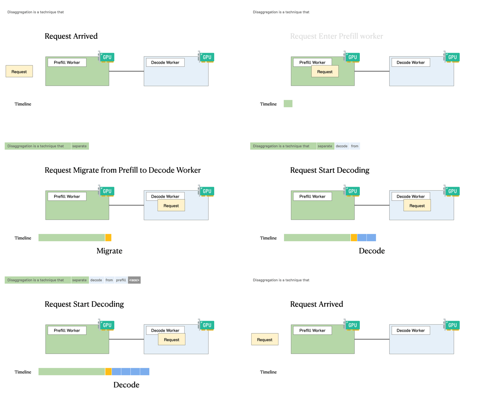
The DistServe team from Hao AI Lab published a short animation of that lifecycle (Figure 3): a request arrives, a prefill worker materializes the KV cache, then a decode worker streams tokens. The clip uses a disaggregated layout; the point here is the phase handoff, not the worker topology.
3.2 Phase 1: Prefill
Prefill is the parallel pass over the prompt; TTFT is the elapsed real time until that pass emits the first token. Every prompt token is processed together (e.g., 4K system + 2K context + 500 query) in one forward.
As called out earlier, Prefill is compute-bound, and it helps to see why by naming what attention actually does. Each token is turned into three vectors: a query (what this token is looking for), a key (what it offers to be matched on), and a value (the content it hands over when matched). Attention scores every token’s query against every token’s key, and those scores decide how much of each token’s value flows where.
“Every query against every key” is the load-bearing phrase. With a prompt of $L$ tokens we have $L$ queries and $L$ keys, so the model computes a score for all $L \times L$ pairs in one pass:
$$ \text{attention FLOPs} \propto L^{2} \cdot d $$
where $d$ is the head dimension, the length of each query and key vector, so each of the $L^{2}$ scores costs about $d$ multiply-adds.
Why does it matter? Doubling $L$ roughly quadruples attention work ($2L)^{2} = 4L^{2}$, while the dense linear layers, the per-token feed-forward matmuls that touch each token on its own, only double. As prompts get longer, runtime shifts from dense matrix multiplies (roughly linear in $L$) to attention (quadratic in $L$), which becomes the bottleneck. This $L^{2}$ scaling is the conventional full-attention baseline; hybrid-attention designs (including DeepSeek V4’s, which mixes sparse and compressed attention to cut prefill FLOPs and KV) are built specifically to bend that curve, so read the quadratic as the cost these architectures are attacking, not a universal law.
The numbers below are indicative, measured on Llama-3.1-70B on a single H100-class GPU; our hardware and batching will shift them depending on the model, precision, and GPU. The point is the shape of the scaling, not the absolute milliseconds.
| Input length (tokens) | TTFT (time to first token) |
|---|---|
| 1K | ~18ms |
| 8K | ~72ms |
| 32K | ~472ms |
| 122K | ~2,200ms |
The scaling is super-linear once prompts get long: below about 8K the linear dense-layer term still dominates, so 1K to 8K grows roughly in proportion to length, but the jump from 8K to 32K is more than 4× because the quadratic attention term takes over. Until prefill finishes, the user sees nothing: that wait is TTFT.
Prefill and decode differ first in the shape of the work (Figure 4): prefill scores every prompt token against every other, while decode scores only the newest token against the whole cache.

3.3 Phase 2: Decode
Once prefill finishes and the first token is emitted, decode takes over. As we touched on earlier, generation is autoregressive: each new token conditions on all previous tokens plus the growing KV cache, so token 57 cannot start until token 56 exists.
Decode is memory-bandwidth-bound at low batch. For a single sequence, step time is dominated by reading weights from HBM, not by the matmul FLOPs. The two timings below make that ratio concrete for a 70B dense model in FP16 at batch size 1 on an H100-class GPU, under two simplifying assumptions: that the weights are streamed once per step, and that KV traffic is negligible at short context.
Question 1: how long does it take to stream the weights once?
To stream the weights, we must first know how many bytes they are. The model has $N = 70 \times 10^9$ parameters, and FP16 stores 2 bytes per parameter, so the total weight footprint is $70 \times 10^9 \times 2\ \text{bytes} =$ 140 GB.
Every decode step must pull that working set from HBM:
$$ T_{\text{mem}} \approx \frac{N \cdot \text{bytes/param}}{B_{\text{HBM}}} = \frac{140\ \text{GB}}{3.35\ \text{TB/s}} \approx 42\ \text{ms} $$
Reading this formula left to right: the numerator is the total bytes to move (140 GB), and the denominator is how fast HBM can move them (3.35 TB/s). The result is approximately 0.042 seconds ($140 / 3350 \approx 0.042$), or 42 milliseconds. This is an idealized lower bound on TPOT at batch size 1: at peak HBM bandwidth on a single GPU, we cannot emit the next token faster than HBM can deliver the weights, regardless of how many FLOPs the datasheet advertises. Real deployments sit above it (tensor parallelism, quantization, and less-than-peak bandwidth all move the number), but this bound is what makes decode bandwidth-bound in the first place.
One convention for the rest of Part I: every number here uses an H100-class GPU (3.35 TB/s HBM) as a single fixed reference point. The two-node box in the opening ran on H200s (4.8 TB/s), roughly 1.4× more bandwidth, which scales these milliseconds down proportionally and raises the absolute $B^{\star}$; it moves the numbers, not the shape of the argument or where the crossover logic lands.
Question 2: how long would the math take if bandwidth were free?
The dominant work is matrix-vector multiplies over the weights. Counting a multiply-add as 2 FLOPs, a dense forward is about $2N$ FLOPs per token (one multiply and one add per parameter, roughly). If we use the H100’s BF16/FP16 tensor-core peak (~989 TFLOP/s), instead of the FP8 peak, we get the compute time as follows:
$$ T_{\text{compute}} \approx \frac{2 \cdot N}{\text{peak FLOP/s}} = \frac{140 \times 10^9}{0.989 \times 10^{15}} \approx 0.14\ \text{ms} $$
Same $N$, but now the numerator is FLOPs, and the denominator is peak FLOP/s. The $2$ is the multiply-add; the $140 \times 10^9$ is $2N$ written as FLOPs. Check: $1.4 \times 10^{11} / 9.89 \times 10^{14} \approx 1.4 \times 10^{-4}$ s ≈ 0.14ms.
What does the ratio mean? Decomposing the step time into memory and compute, we see that the GPU spends ~300× more time waiting on HBM than doing math:
$T_{\text{mem}} / T_{\text{compute}} \approx 42 / 0.14 \approx 300\times$
In other words, for every millisecond of useful math, the GPU spends ~300ms waiting on HBM. The SMs (Streaming Multiprocessors, the GPU’s main compute blocks) are mostly idle. We can also see it as arithmetic intensity at batch 1:
$$ I_{\text{decode},,B{=}1} \approx \frac{2N\ \text{FLOPs}}{N \cdot b\ \text{bytes}} = \frac{2}{b} = 1\ \text{FLOP/byte (FP16)} $$
The chip wants ~300 FLOPs/byte (next subsection); we are delivering ~1, a ~300× shortfall. One thing worth flagging so it doesn’t trip us up: this ~300× and the ~300× time ratio from just above ($42/0.14$) land on the same number by coincidence, not for the same reason. One is FLOPs-per-byte, the other is milliseconds against milliseconds; they measure different things and only happen to be close on this hardware, so don’t read a shared cause into it.
That shortfall is why single-stream decode at batch size 1 wastes almost all of the GPU, and it is exactly what batching fixes. Reading the weights out of HBM is the expensive step, and it costs the same whether we run one sequence or a hundred. So if we push more sequences ($B$) through a single weight load, each extra one is nearly free: the useful math on top grows with $B$ while that one weight read stays fixed, and intensity climbs back toward the ~300 the chip actually wants.
Figure 5 is the phase split in one picture:

Almost every optimization in the rest of this post pulls on one of those two boxes (prefill or decode) or on the KV handoff between them. Figure 6 sorts the main levers into those three buckets:

On the decode side, batching is the key lever: at $B=1$ we underuse the GPU, naive static batching wastes work on padding, and continuous batching keeps $B$ high with less waste.
3.4 Putting both phases on the roofline
That 42ms weight stream against 0.14ms of math is one instance of the question every accelerator workload poses: is this step bound by memory or by compute, and what batch size moves us across the line between them?
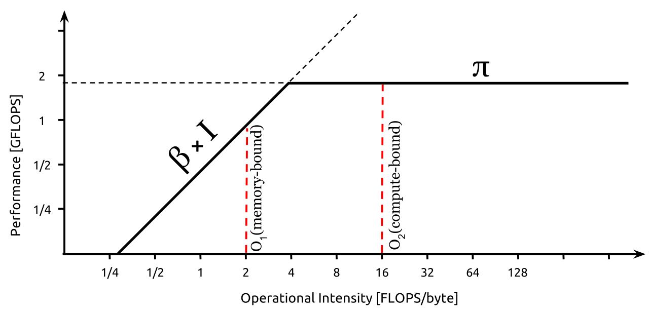
The standard tool is the roofline model (Williams, Waterman, and Patterson, 2009): attainable performance (FLOPs/s) against arithmetic intensity (FLOPs per byte from HBM). Prefill and decode land on opposite sides of the ridge; treating “GPU latency” as one scalar collapses that distinction.
- On the left, the sloping line is the memory roof: performance ≤ bandwidth × intensity. If we don’t do enough math per byte loaded, we are stuck waiting on HBM.
- On the right, the flat line is the compute roof: performance ≤ peak FLOPs/s. Once intensity is high enough, more bandwidth doesn’t help; the ALUs are the limiter.
- Where the two lines meet is the ridge point. To the left of it we’re memory-bound; to the right we’re compute-bound. Figure 7 is the classic picture:

Now drop the two inference phases onto that same roofline (Figure 8):
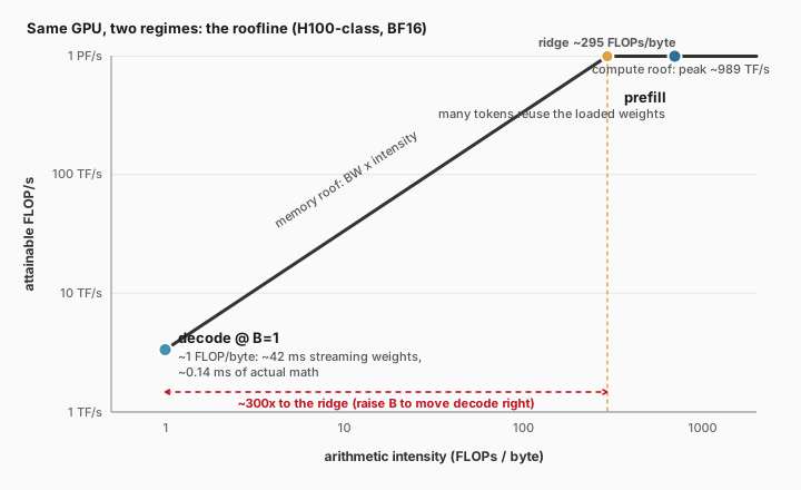
Prefill processes many tokens in one pass, so the loaded weights get reused heavily: high intensity, compute-bound, right side of the roof. Decode at batch 1 loads ~140 GB of weights to do ~0.14ms of math: extremely low intensity, memory-bound, deep on the left.
In practice, each decode step finishes when both the math and the memory traffic are done, so wall-clock is the slower of the two:
$$ T_{\text{step}} \approx \max{t_{\text{compute}}, t_{\text{mem}}} + t_{\text{overhead}} $$
Read the formula as three things that the step pays: the compute time, the memory-move time, and a fixed overhead (launch, scheduling, sync, communication). Compute and memory overlap, so only the slower of the two counts; overhead is then added on top. With memory at 42ms and compute at 0.14ms, memory swamps everything, which is why faster ALUs alone barely move TPOT.
Questions 1 and 2 back in section 3.3 pinned the two costs at batch 1: about 42ms of memory against 0.14ms of math. The next three questions scale that up to a real batch and find where the two costs finally meet.
Question 3: As we add sequences to the batch, how do compute time and memory time each change?
Put $B$ sequences through the same forward pass, and the two costs become:
$$ t_{\text{compute}} \approx \frac{2 \cdot B \cdot N_{\text{active}}}{\text{peak FLOP/s}}, \qquad t_{\text{mem}} \approx \frac{N_{\text{total}} \cdot b + B \cdot L \cdot m_{\text{KV/token}}}{\text{peak bandwidth}} $$
Let us break this down and understand:
- $t_{\text{compute}}$ is the per-token work ($2 N_{\text{active}}$ FLOPs) done once for each of the $B$ sequences, divided by the compute ceiling.
- $t_{\text{mem}}$ splits in two: a fixed weight read ($N_{\text{total}} \cdot b$) plus a KV read ($B \cdot L \cdot m_{\text{KV/token}}$) that grows with both batch and context, all divided by the bandwidth ceiling.
| Symbol | Meaning |
|---|---|
| $B$ | Decode batch: concurrent sequences sharing one forward pass |
| $N_{\text{active}}$ | Parameters that fire for a token (all of them on dense; a fraction on MoE) |
| $N_{\text{total}}$ | Parameters whose bytes we still fetch (experts included when they sit in the working set) |
| $b$ | Bytes per parameter (2 for FP16, 1 for FP8) |
| $L$ | Context length in tokens |
| $m_{\text{KV/token}}$ | KV cache bytes per token (model-dependent; ~320 KB for the Llama-3.1-70B FP16 GQA example worked in Part 3 ) |
The formulas hide two facts that drive every batching decision:
- Weight fetch is fixed, no matter how large $B$ gets. The $N_{\text{total}} \cdot b$ term costs the same for 1 sequence or 100: one weight load feeds the whole batch. That fixed cost, spread over more sequences, is the free lunch batching buys.
- KV fetch and compute both scale with $B$. Each added sequence brings its own KV bytes and its own FLOPs, so $t_{\text{compute}}$ climbs linearly while $t_{\text{mem}}$ climbs only through its KV term.
Net effect: batching keeps paying off while that fixed-weight read dominates, then flattens once the growing KV traffic and compute catch up.
Question 4: how much math must we do per byte fetched to keep the GPU busy?
Set KV aside for a moment. The ridge intensity, the break-even point where memory-bound flips to compute-bound, is simply peak compute divided by peak bandwidth:
$$ I_{\text{ridge}} = \frac{\text{peak FLOP/s}}{\text{peak bandwidth}} = \frac{989\ \text{TFLOP/s}}{3.35\ \text{TB/s}} \approx 295\ \text{FLOPs/byte} $$
Read it as a spending budget: on this GPU, every byte we pull from HBM buys about 300 FLOPs of BF16 tensor-core work. Do fewer than ~300 FLOPs per byte and the ALUs sit idle waiting on memory; do more and bandwidth sits idle waiting on the ALUs. That is exactly the batch-1 story from earlier: intensity was ~1 FLOP/byte against a chip that wanted ~300, a 300× gap.
Question 5: how many sequences must we batch before decode stops being bandwidth-bound?
Decode hits the crossover when compute time and memory time are equal. Keep only the weight term (drop KV for a clean lower bound), set the two equal, and solve for $B$:
$$ \frac{2 \cdot B \cdot N_{\text{active}}}{\text{peak FLOP/s}} = \frac{N_{\text{total}} \cdot b}{\text{peak bandwidth}} $$
Rearrange:
$$ B = \frac{\text{peak FLOP/s}}{\text{peak bandwidth}} \cdot \frac{b}{2} \cdot \frac{N_{\text{total}}}{N_{\text{active}}} = I_{\text{ridge}} \cdot \frac{b}{2} \cdot \frac{N_{\text{total}}}{N_{\text{active}}} $$
For FP16, $b = 2$, so $b/2 = 1$ and the factors cancel cleanly:
$$ B^{\star} \gtrsim I_{\text{ridge}} \cdot \frac{N_{\text{total}}}{N_{\text{active}}} \approx 300 \cdot \frac{N_{\text{total}}}{N_{\text{active}}} $$
What $B^{\star}$ means in practice. Read it as a tipping point: the decode batch size where the fixed cost of reading the weights out of HBM is finally matched by the compute stacked on top. The two sides behave in opposite ways:
- Below $B^{\star}$, we are bandwidth-bound. The weight read dominates the step, and it costs the same whether one sequence shares it or a hundred. So each extra sequence rides that same weight stream almost for free: throughput climbs while the per-step time barely moves.
- Above $B^{\star}$, we are compute-bound. The free ride is over. Compute (and the KV traffic that grows with the batch) is now the limiter, so every added sequence starts costing real time.
We rarely get to sit exactly at $B^{\star}$ in production, because latency SLOs and KV-cache capacity usually cap the batch first. But knowing roughly where it sits answers the one question that matters: do we still have bandwidth headroom to add sequences, or have we already tipped into compute-bound territory?
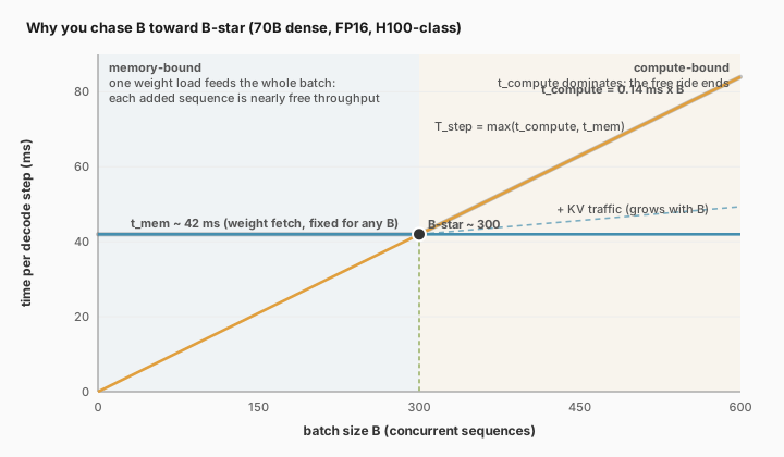
Figure 9 plots both costs against batch size: a flat weight-fetch (memory) line that stays put as the batch grows, and a compute line that rises with every added sequence. Where they cross is $B^{\star}$, with the memory-bound region to its left and the compute-bound region to its right.
Dense vs. MoE. The ratio $N_{\text{total}}/N_{\text{active}}$ is what makes MoE behave differently here.
- Dense model: every parameter fires on every token, so $N_{\text{total}} = N_{\text{active}}$, the ratio is 1, and $B^{\star}$ lands at a few hundred. That is the familiar “decode intensity ≈ batch size” rule of thumb (at FP16, FLOPs/byte ≈ $B$).
- MoE: only a slice of the parameters fires per token, but the engine still has to fetch the whole active expert working set from HBM. So it pays close to the full weight-read cost while doing only a fraction of the math, and that mismatch is the ratio.
DeepSeek V4-Pro makes the gap concrete: it activates roughly 49B of its 1.6T parameters per token (from section 1), about a $33\times$ ratio once the always-on attention and shared expert are folded in. Plug that in and $B^{\star} \gtrsim 300 \times 33 \approx 10{,}000$ concurrent sequences before the weight fetch pays for itself.
Treat that 10,000 as a direction, not a sizing target. It explains why wide-EP serving is so hungry for batch, but the real crossover is messier than a single-GPU weight-stream sum:
- Under expert parallelism, each GPU holds only some experts and reuses those local weights across whatever tokens get routed to it. So the true crossover depends on how many experts sit on each rank, how evenly the router spreads tokens, and what the all-to-all costs, none of which show up in this back-of-envelope number.
- We never get to sit at $B^{\star}$ anyway: KV-cache capacity and latency SLOs cap the batch well before we reach it.
That is the whole reason frontier MoE serving works so hard to build a large effective batch by other means: disaggregation, big KV budgets, and expert parallelism.
Three consequences fall out of the same roofline:
- A hard floor on step time. Each decode step must stream the active weights from HBM at least once, so step time cannot drop below model-bytes / bandwidth (the ~42ms weight-stream bound for this 70B FP16 example). Single-stream decode therefore has a physical floor of tens of milliseconds per step, no matter how many FLOPs the GPU has.
- Which hardware helps depends on the phase. When decode is memory-bound, bandwidth is the cap and more peak FLOPs do nothing. (An H200 keeps the H100’s Hopper FLOPs but adds far more HBM capacity, 80 → 141 GB, than bandwidth, 3.35 → 4.8 TB/s: capacity unlocks bigger batches and longer KV, bandwidth sets the decode floor.) When prefill is compute-bound, compute is the cap, and that is finally where the FLOPs we paid for get used.
- Why output tokens cost more. The same physics shows up on the price sheet: output tokens are typically several times pricier than input tokens because decode is memory-bound (low MFU, Model FLOPs Utilization: the fraction of peak math we actually use) while prefill is nearer compute-bound. Cached input tokens (prefix hits) are cheaper still, because replaying stored KVs beats recomputing them.
Where every optimization lands. Every architecture move later in the series (the levers in Figure 6) is ultimately a way to buy more useful FLOPs per byte fetched: slide decode rightward toward the crossover, or keep a compute-bound prefill from stalling it.
Note: Reasoning models turn a short prompt into a long decode of thinking tokens. Prefill stays short, so dialing effort up is mostly dialing how long we stay memory-bound.
3.5 The interference problem
As we have seen, Prefill is compute-bound, and decode is bandwidth-bound: opposite regimes on the same silicon. Interference is what happens when they share one GPU’s timeline: a compute-bound prefill steals steps from the bandwidth-bound decode streams already in flight. The trap is that average throughput can still look healthy while P99 TPOT quietly collapses under mixed traffic.
The concrete picture (Figure 10): a user submits a long prompt of 4K tokens, and their prefill takes around 300ms. During those 300ms, every other in-flight decode request is blocked: none can advance because the GPU is busy with the new request’s prefill. Their TPOT spikes.
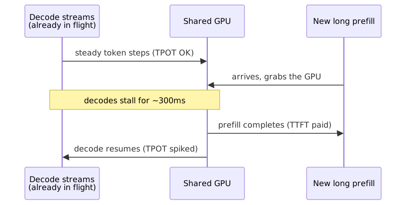
DistServe’s measurements quantify this effect: a single large prefill can inflate TPOT for concurrent requests by an order of magnitude or more (DistServe measured up to 30×), depending on the distribution of prompt lengths.
4. Running prefill and decode on one GPU: continuous batching
Decode throughput climbs when we raise concurrent sequences $B$ toward $B^{\star}$, because one weight load then serves many tokens. Prefill/decode interference is what happens when those sequences share a GPU badly. So the scheduler question is not “should we batch?” It is how we form $B$, how we keep it full under variable output lengths, and what we do when a new prefill wants into an in-flight decode step.
4.1 Why batch, and what static batching got wrong
Without batching, each request runs alone ($B=1$). Every decode step streams the full weight working set from HBM for a single token. For the 70B FP16 example above, that is ~42ms of memory time against ~0.14ms of math: the SMs sit underfed, tensor cores idle, and TPOT is dominated by bandwidth. Arithmetic intensity never approaches the ~300 FLOPs/byte crossover, so we never reach the compute-bound regime. Latency for that one user can look fine; fleet tokens/s and $/token look terrible.
Batching means running multiple sequences through the same forward so one weight fetch (and one kernel launch sequence) produces a token for each of them. That is the serving-side move that raises arithmetic intensity and amortizes $t_{\text{mem}}$. The costs are real: requests queue until a batch forms, mixed prompt/output lengths make the step look like the worst case in the batch, and a long prefill in the mix stalls everyone else’s decode (section 3.5).
Static batching was the first widely deployed answer (pre-ORCA / pre-vLLM). The server collects $N$ requests, forms a batch, runs that batch until every request has finished generating, and only then admits new work. Cooperative multitasking: no slot frees until the longest sequence in the cohort completes.
Versus no batching, static batching is a clear win whenever $N$ is large, and lengths are similar: we finally get $B>1$ and ride toward $B^{\star}$.
The failure mode shows up under realistic length skew. Picture a batch of ten requests where one generates 2,000 tokens and the other nine generate 10 each:
- The nine short requests finish after 10 steps, but their slots stay locked until the long one finishes at step 2,000.
- For steps 11 through 2,000, those nine slots do nothing but padding (masked no-ops), spending compute on throwaway work.
- New requests wait behind the whole cohort. Even a five-step request cannot start until step 2,000.
Utilization collapses and head-of-line blocking dominates. Moving off this run-to-completion policy to iteration-level scheduling is exactly the change the ORCA paper (Yu et al., OSDI 2022) measured at up to 36.9× throughput over NVIDIA FasterTransformer on GPT-3 175B, at a matched latency target on their benchmark setup.
4.2 Continuous batching: iteration-level scheduling
Static batching’s whole problem was the cohort: once the batch forms, it is frozen until the last sequence finishes. Continuous batching removes that constraint with one small change to when the scheduler is allowed to act, and it is the policy at the heart of vLLM and every modern serving engine.
The core idea. Continuous batching (iteration-level scheduling) keeps the amortization win of $B>1$ but drops the padding tax that sinks static batching. The difference is where the scheduling decision happens:
- Static batching decides the batch once and holds it until the whole cohort drains.
- Continuous batching re-decides at every decode step: it drops any sequence that just finished, pulls a waiting request into the freed slot, and runs the next step on that new mix.
Nobody waits for the longest sequence, because the batch is never locked to a cohort in the first place. It is reassembled token by token.
Why this is not mid-kernel preemption. The word “step” is doing the load-bearing work: the swap happens between steps, never inside one. A running kernel is never interrupted; the scheduler just gets a fresh say each time the GPU comes up for air. So it is closer to a connection pool handing an idle connection to the next caller than to preempting a thread that is still running.
The one residual cost: admission. Inserting a new request means running its prefill inside a decode step. That spikes $t_{\text{compute}}$ for the whole iteration, which is section 3.5’s interference problem showing up at the scheduler boundary. We are still holding $B$ near $B^{\star}$ to keep $t_{\text{compute}}$ and $t_{\text{mem}}$ balanced, so every admission briefly pulls the step back toward compute-bound. Figure 11 shows what each scheduler does at every step:

That is the control logic. Figure 12 shows the same two policies playing out over time: static batching leaves finished-but-padded slots idle until the longest sequence in the cohort completes, while continuous batching refills each slot the moment it frees.
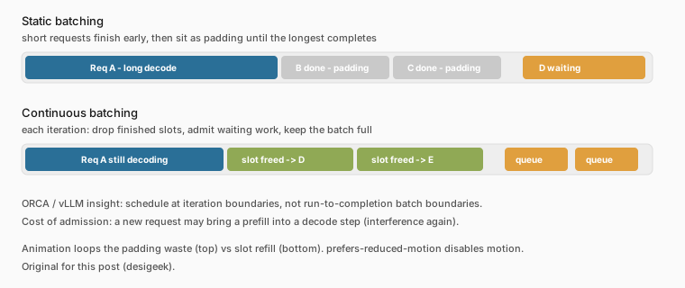
Chunked prefill and disaggregation later attack the admission/interference residual that continuous batching does not remove.
One caveat: everything so far assumes online serving, where a latency SLO caps how big the batch can grow. Offline batch inference is the happy mirror image. When there is no user waiting, nothing stops us from parking the batch right at or above $B^{\star}$ and running flat-out for throughput. That is why the very same GPU that looks bandwidth-starved serving live traffic can finally saturate its compute on an overnight batch job: the latency budget that held the batch small during the day is simply gone.
Part 1 recap. The whole part comes down to a few linked ideas:
- A request is two workloads on one GPU. Prefill processes the prompt in one compute-heavy pass and sets our first-token latency (TTFT). Decode then emits tokens one at a time, waiting mostly on memory, and sets our per-token latency (TPOT).
- Each decode step runs at the speed of its slower half, math or memory. At batch size 1 that half is almost always memory: roughly 42ms spent streaming weights to do about 0.14ms of math.
- Batching is the fix. Pushing more sequences through a single weight load raises the useful math done per byte fetched, up to a crossover batch size ($B^{\star}$) where compute finally catches memory. Below it, each added sequence is nearly free; above it, it costs real time. For a dense model that point is a few hundred sequences; for a large MoE it is far higher.
- Continuous batching keeps us near that point in practice. It refills each slot the moment a sequence finishes, rather than freezing a whole cohort and paying the static-batching padding tax, all while staying inside our latency SLO.
Keep reading
Part 1 of 3. Next up, Part 2 · Below Python
: what actually runs under vllm serve, the GPU, the kernels, and the compilers where the bug actually lived, and why --enforce-eager and disabling torch.compile couldn’t touch it.
- Part 1 (this post) · Physics of a request
- Part 2 · Below Python
- Part 3 · Serving at scale
References & Further Reading
Grouped by topic; starred (★) entries are the best starting points. These cover Part 1; Parts 2 and 3 carry their own reference blocks.
The “why this is hard” overview
- ★ Making Deep Learning Go Brrrr From First Principles (Horace He) , the single best popular treatment of compute-bound vs. memory-bound vs. overhead-bound.
- ★ Inside vLLM: Anatomy of a High-Throughput LLM Inference System (Aleksa Gordić)
- ★ The Inference Engineering Masterclass (Philip Kiely and Ali Taha, Baseten × Latent Space, 2026) , a practitioner tour of quantization, speculators, disaggregation, and the nondeterminism war stories this series draws on.
- Inference Engineering (Philip Kiely, Baseten) , a book-length companion to the same material.
- For a given model, inference speed comes down to four things (Lan Chu) , compact vocabulary card for compute / capacity / bandwidth / serving
- Roofline: an insightful visual performance model for floating-point programs (Williams, Waterman, Patterson, 2009)
- How GPT, Claude, and Gemini are actually trained and served (Reiner Pope with Dwarkesh Patel) , blackboard walkthrough of ridge / $B^{\star}$ / pricing-as-physics for serving cost
- Reiner Pope flashcards (Dwarkesh) , drill set for the batch-size and memory-time equations used on the ridge above
- Transcript gist of the same episode
Prefill and decode phases
- ★ Prefill vs Decode: LLM Inference Phases Explained (Redis)
- Deep dive into Text Generation Inference with LLMs (Hugging Face)
- DistServe: Disaggregating Prefill and Decoding for Goodput-optimized LLM Serving (Zhong et al., OSDI 2024)
- ★ Throughput is Not All You Need / DistServe blog (Hao AI Lab @ UCSD)
- Splitwise: Efficient Generative LLM Inference Using Phase Splitting (Patel et al., ISCA 2024)
Continuous batching and scheduling
- ORCA: A Distributed Serving System for Transformer-Based Generative Models (Yu et al., OSDI 2022) , the paper that established the iteration-level scheduling foundation now commonly called continuous batching.
- Taming the Throughput-Latency Tradeoff in LLM Inference with Sarathi-Serve (Agrawal et al., OSDI 2024)
Desigeek series (prerequisites and related posts)