Over the last several benchmark cycles, I kept coming back to the same practical question: once you hold the hardware and methodology constant, which large open models are actually pleasant to serve, which ones merely load, and which ones become operationally awkward the moment you move beyond a demo?
This post is a technical deep dive into that question. Instead of presenting a generic leaderboard, I focus on the details that usually matter in real deployments: throughput under fixed traffic shapes, latency behavior, scaling across 8x and 16x H200 shapes, and the caveats that only show up when you try to run these models end to end.
It also grew out of a public r/LocalLLaMA thread asking what people most wanted to see tested on this hardware. The model set in this post is therefore not just a random grab bag. It reflects the cluster bring-up requests that came up most often, plus the operational work required to turn those requests into comparable benchmark results.
TL;DR
Llama 4 ScoutandMiniMax M2.1were the strongest overall performers in this benchmark set.- In several cases,
8x H200was a better serving shape than16x H200for the same workload mix. DeepSeek V4 Flashwas healthy and interesting, especially on long-context runs.DeepSeek V4 Proonly produced fallback-shape numbers in this April 2026 run because the intendedDP+EPpath was blocked by a router dtype bug ( #40862 ) — fixed upstream in June 2026 ( #43425 ); see §9 update.- A fixed benchmark matrix plus Langfuse validation mattered almost as much as the raw throughput numbers.
1. Hardware and Profiles
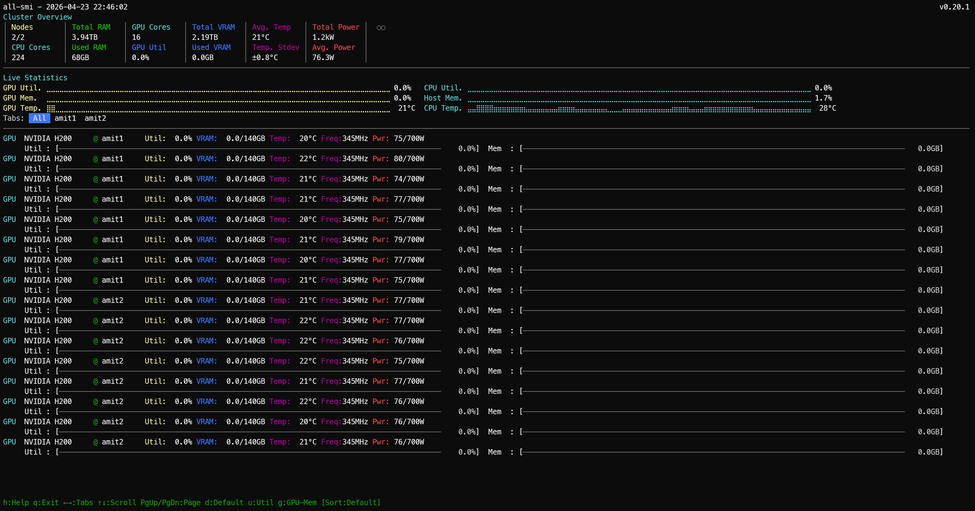
The benchmark environment is a 16 x H200 cluster across two nodes, but the machine shape is important because this is not a generic collection of GPUs. The cluster is built on Dell PowerEdge XE9680L servers, each with 8 x NVIDIA H200, dual Intel Xeon Platinum 8570 CPUs, and 2.0 TiB of system RAM. Each node also carries 8 x 3.84 TB Dell U.2 NVMe drives plus a Dell BOSS-N1 boot device.
On the data-plane side, each node exposes 8 active 400G ConnectX-7 InfiniBand links, which is 3.2 Tb/s of raw InfiniBand link rate per node, along with 2 active 200G BlueField-3 / ConnectX-7 Ethernet links. So at the cluster level, this is roughly 2.30 TB of aggregate HBM, 4.0 TiB of host RAM, and a genuinely fast multi-rail fabric rather than a generic dual-server setup.
For this study, the primary serving runtime is vLLM, and the benchmark profiles are intentionally fixed so the comparisons do not drift from one model to the next. Every model was measured against the same three workload profiles:
1024 in / 256 out / concurrency 11024 in / 256 out / concurrency 168192 in / 256 out / concurrency 4
For anyone new to this notation:
1024 inmeans each request starts with a prompt of about 1024 input tokens.256 outmeans each request is allowed to generate up to about 256 output tokens.concurrency Nmeans how many requests are in flight at the same time.
What each target represents in practice:
| Target | What it represents |
|---|---|
1024 in / 256 out / concurrency 1 | Single-user responsiveness (best for reading latency and per-token decode behavior). |
1024 in / 256 out / concurrency 16 | Loaded serving throughput (best for seeing how well the model holds up under parallel demand). |
8192 in / 256 out / concurrency 4 | Long-context behavior (best for testing heavier prompt processing with moderate parallelism). |
Throughout the post, results are labeled with shorthand profile names that encode the same information:
| Profile shorthand | Meaning |
|---|---|
latency-1024x256-c1 | Single-user latency profile (1024 input tokens, 256 output tokens, concurrency 1). |
serve-1024x256-c16 | Loaded serving throughput profile (1024 input tokens, 256 output tokens, concurrency 16). |
longctx-8192x256-c4 | Long-context profile (8192 input tokens, 256 output tokens, concurrency 4). |
Where a model was tested on multiple hardware shapes, the suffix -16x (or -8x) is appended to the profile name to indicate which shape that row covers, e.g. latency-1024x256-c1-16x means the latency profile run on the 16x H200 shape.
Later tables also use runtime topology labels such as TP, PP, DP, and EP. These describe how the model was distributed across GPUs during serving:
TP= tensor parallelism, meaning tensor operations are split across multiple GPUsPP= pipeline parallelism, meaning different layers or blocks are split into sequential pipeline stagesDP= data parallelism, meaning multiple replicas process different requests in parallelEP= expert parallelism, meaning MoE experts are distributed across GPUs
So TP=8, PP=2 means the model was served with 8-way tensor parallelism and 2 pipeline stages, which typically implies a 16-GPU deployment shape for that run.
The results tables in each model section report three metrics alongside the profile label:
Output tok/s— aggregate output throughput across all concurrent requests. This is the headline number: how many tokens per second the serving stack is generating in total under that workload shape.TTFT (ms)— time to first token. How long from when the request was sent until the first output token arrived back. Lower is better. TTFT reflects prefill time, KV cache allocation, and scheduling overhead combined, and it is the number that determines how responsive the model feels to a user waiting for a reply.TPOT (ms)— time per output token. The average time between consecutive output tokens after the first one. Lower is better. TPOT reflects decode speed and is what determines whether a streaming response feels smooth or choppy once it starts.
The reason all three matter together: a model can post high aggregate tok/s at c16 but still have a painful user experience if TTFT is high, because every user waits that long before seeing any output. Conversely, a model with modest tok/s but low TPOT can feel snappier than the numbers suggest.
The model list below is presented in no particular order. These are the large open models that were both available and runnable during the benchmark window, spanning a mix of architectures, training approaches, and quantization formats. It is not an exhaustive survey of the open-model ecosystem, but it is a practical cross-section of the models people are actively evaluating and that I could run with enough stability to generate comparable results.
Qwen/Qwen3-235B-A22B-Instruct-2507moonshotai/Kimi-K2.6deepseek-ai/DeepSeek-V4-Flashdeepseek-ai/DeepSeek-V4-Prometa-llama/Llama-4-Scout-17B-16E-Instructzai-org/GLM-5.1-FP8MiniMaxAI/MiniMax-M2.1mistralai/Mistral-Large-3-675B-Instruct-2512
The goal was straightforward: one fixed benchmark suite, one cluster, several large open models, and enough implementation detail that the results are useful beyond this specific environment.
2. Method
All of the vLLM runs use the same serving profiles and the same result format. Each saved result includes the exact model name, prompt length, output length, concurrency, request rate, hardware label, engine, and timestamp. That consistency matters because a standalone “tokens per second” number stops being useful the moment people start changing prompt length, output length, or concurrency and still try to compare the outcome directly.
Not every model ran on the same vLLM build, and that was deliberate rather than inconsistent. The default lane was the stable v0.19.1 release. The exceptions were models where the generic stable image was either not the supported path, not feature-complete enough for that model’s runtime requirements, or not what the model vendor’s integration expected:
- GLM-5.1-FP8 used
v0.19.1.dev1— the FP8 and multi-node bring-up path for GLM required a newer-than-stable build to work cleanly. - MiniMax M2.1 used
v0.19.1rc1.dev203via thevllm/vllm-openai:minimax27image — MiniMax ships its own official runtime lane with MiniMax-specific parser and expert-parallel behavior; the stock image is not the right lane for this model. - DeepSeek V4 Flash and V4 Pro both used
vllm/vllm-openai:deepseekv4-cu130— DeepSeek V4 requires the dedicated CUDA image; the generic image is not the supported serving path.
The short version: deviations happened only when the model or runtime integration required a special lane. Where the engine lane affected the result, it is noted in the model-specific metadata block.
2.1 Langfuse
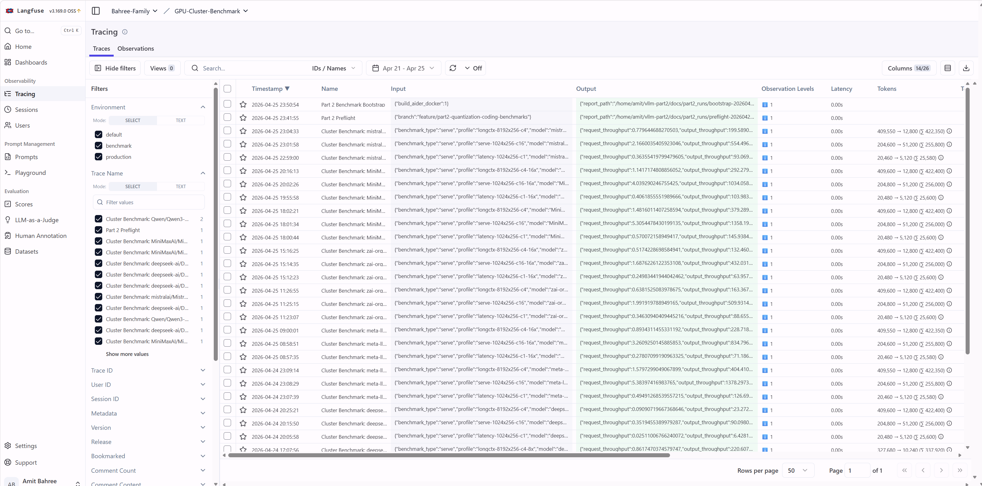
Langfuse is the observability layer I used to verify that a run was genuinely healthy from end to end. In other words, the bar was not merely “the server came up” but “the model served requests correctly, produced output, and emitted traces that matched the saved benchmark artifacts.”
Each run emitted traces tagged with model identity, profile (c1, c16, c4), and hardware shape. Those traces served as a cross-check against the saved result files. Only runs with both complete result files and successful traces were counted as comparable in the summary tables.
3. Quick Comparison (Throughput-First)
If you want the numbers before the per-model context, this is the place to start. The tables and charts below cover all comparable runs side by side.
3.1 Top 3 by Output Throughput (tok/s) per Profile
The table below answers a simple question: which model led each workload profile? Each profile represents a different traffic shape, so the rankings should be interpreted within a profile rather than across profiles. Higher output tok/s means more generated tokens per second across all in-flight requests.
| Profile | #1 (highest tok/s) | #2 | #3 |
|---|---|---|---|
latency-1024x256-c1 | MiniMax M2.1 (145.94 tok/s) | Llama 4 Scout (126.70 tok/s) | Mistral Large 3 (93.07 tok/s) |
serve-1024x256-c16 | Llama 4 Scout (1378.30 tok/s) | MiniMax M2.1 (1358.19 tok/s) | Qwen 235B (643.56 tok/s) |
longctx-8192x256-c4 | Llama 4 Scout (404.41 tok/s) | MiniMax M2.1 (379.29 tok/s) | DeepSeek V4 Flash (220.59 tok/s) |
3.2 Completed Runs Side-by-Side (Output Throughput)
Where the Top 3 table highlights the leaders, this table shows the full completed field so every model can be compared across the same three benchmark profiles at once. The values here are output throughput (tok/s), and the Notes column captures important caveats such as fallback topologies.
| Model | Hardware shape used | c1 tok/s | c16 tok/s | c4 tok/s | Notes |
|---|---|---|---|---|---|
| Llama 4 Scout | 8x H200 | 126.70 | 1378.30 | 404.41 | Best overall in this fixed profile mix |
| MiniMax M2.1 | 8x H200 | 145.94 | 1358.19 | 379.29 | Fastest c1 profile |
| Mistral Large 3 | 8x H200 | 93.07 | 554.50 | 199.59 | Stable baseline, mid-pack throughput |
| GLM-5.1-FP8 | 8x H200 | 88.66 | 509.93 | 163.37 | 16x scaling regressed |
| DeepSeek V4 Flash | 8x H200 | 69.96 | 543.13 | 220.59 | 8x helps mostly on long-context |
| Kimi K2.6 | 16x H200 | 64.38 | 470.52 | 179.45 | Stable completed run |
| Qwen 235B | 16x H200 | 56.46 | 643.56 | 170.47 | Stable completed run |
| DeepSeek V4 Pro | 8x H200 fallback (TP=8, eager) | 6.43 | 90.10 | 23.27 | April run: intended DP+EP blocked; fixed upstream Jun 2026 |
The three charts below show output throughput (tok/s) for all models, split by workload profile so each chart can use an appropriate scale.
What each chart presents:
c1(latency-1024x256-c1): single-user responsiveness at concurrency1c16(serve-1024x256-c16): loaded serving throughput at concurrency16c4(longctx-8192x256-c4): long-context behavior with8192-token prompts at concurrency4
Single-user latency (c1) - output tok/s, all models
xychart-beta
  title "latency-1024x256-c1: output tok/s (higher = better)"
  x-axis ["MiniMax M2.1", "Llama 4 Scout", "Mistral L3", "GLM-5.1-FP8", "DS Flash", "Kimi K2.6", "Qwen 235B", "DS Pro*"]
  y-axis "output tok/s" 0 --> 160
  bar [145.94, 126.70, 93.07, 88.66, 69.96, 64.38, 56.46, 6.43]
Loaded serving throughput (c16) - output tok/s, all models
xychart-beta
  title "serve-1024x256-c16: output tok/s (higher = better)"
  x-axis ["Llama 4 Scout", "MiniMax M2.1", "Qwen 235B", "Mistral L3", "DS Flash", "GLM-5.1-FP8", "Kimi K2.6", "DS Pro*"]
  y-axis "output tok/s" 0 --> 1500
  bar [1378.30, 1358.19, 643.56, 554.50, 543.13, 509.93, 470.52, 90.10]
Long-context (c4) - output tok/s, all models
xychart-beta
  title "longctx-8192x256-c4: output tok/s (higher = better)"
  x-axis ["Llama 4 Scout", "MiniMax M2.1", "DS Flash", "Mistral L3", "Kimi K2.6", "Qwen 235B", "GLM-5.1-FP8", "DS Pro*"]
  y-axis "output tok/s" 0 --> 450
  bar [404.41, 379.29, 220.59, 199.59, 179.45, 170.47, 163.37, 23.27]
* DS Pro ran on a fallback topology (TP=8, --enforce-eager) - see the DeepSeek V4 Pro section for context.
4. Model Status Snapshot
Most models completed cleanly, but a few required fallback topologies or other caveats that materially change how their results should be interpreted. DeepSeek V4 Pro is the main exception: its published numbers come from a fallback deployment shape (TP=8, --enforce-eager) taken in April 2026 when the intended DP+EP lane failed at startup. That router dtype bug is fixed upstream
as of June 2026 — see §9 for the update and historical context.
| Model | Final status | See section |
|---|---|---|
| Llama 4 Scout (official) | Completed (8x + 16x tested) | Section 5 |
| Llama 4 Scout (unsloth) | Blocked / unreliable | Section 5 note |
| MiniMax M2.1 | Completed (8x + 16x tested) | Section 11 |
| Mistral Large 3 | Completed (8x) | Section 12 |
| GLM-5.1-FP8 | Completed (8x + 16x tested) | Section 10 |
| DeepSeek V4 Flash | Completed (deepseekv4-cu130, 4x + 8x tested) | Section 8 |
| DeepSeek V4 Pro | Completed on fallback shape (TP=8, eager) | Section 9 |
| Kimi K2.6 | Completed | Section 6 |
| Qwen 235B | Completed | Section 7 |
5. Llama 4 Official Scout
Llama 4 Scout ended up being one of the clearest scaling tests in the whole post because it ran cleanly on both shapes and produced directly comparable results. The question here is simple: once the benchmark matrix is held constant, does moving from a single-node 8x H200 lane to a two-node 16x H200 deployment actually improve the serving outcome?
Metadata
- model:
meta-llama/Llama-4-Scout-17B-16E-Instruct - engine:
vLLM v0.19.1 - status: completed (
8xand16xlanes)
| Profile | Shape | Output tok/s | TTFT (ms) | TPOT (ms) |
|---|---|---|---|---|
latency-1024x256-c1 | 8x H200 | 126.70 | 103.83 | 7.51 |
serve-1024x256-c16 | 8x H200 | 1378.30 | 396.57 | 9.73 |
longctx-8192x256-c4 | 8x H200 | 404.41 | 368.10 | 8.14 |
latency-1024x256-c1 | 16x H200 (TP=8, PP=2) | 71.19 | 230.68 | 13.20 |
serve-1024x256-c16 | 16x H200 (TP=8, PP=2) | 834.80 | 520.57 | 16.62 |
longctx-8192x256-c4 | 16x H200 (TP=8, PP=2) | 228.72 | 344.43 | 15.57 |
As a reminder, TP=8, PP=2 means the model was served with 8-way tensor parallelism and 2 pipeline stages, which typically implies a 16-GPU deployment shape for that run. That makes this a clean apples-to-apples scaling comparison: the 16x H200 rows show the intended two-node path for this model, the 8x H200 rows show the single-node alternative, and both lanes produced complete benchmark artifacts with matching Langfuse traces.
The result is clear — scaling from 8 to 16 GPUs was not beneficial for Llama 4 Scout on this workload mix:
- the single-request
c1profile got worse - the
c16throughput profile also got worse - the long-context profile only improved slightly on TTFT, while overall throughput and per-token decode still got worse
In practical terms, official Scout is a strong and fully benchmarkable 8x H200 result, but not a good candidate for this 16x H200 serving shape. The separate unsloth Scout lane never produced stable comparable runs, so it is excluded from the cross-model comparison.
6. Kimi K2.6
Kimi K2.6 completed on 16x H200 using the standard vLLM path. Unlike some of the other models in this post, there is no alternate shape comparison here, so the table below should be read as the canonical Kimi reference point.
Metadata
- model:
moonshotai/Kimi-K2.6 - engine:
vLLM v0.19.1 - shape:
16x H200 - status: completed
| Profile | Output tok/s | TTFT (ms) | TPOT (ms) |
|---|---|---|---|
latency-1024x256-c1 | 64.38 | 229.46 | 14.69 |
serve-1024x256-c16 | 470.52 | 421.06 | 31.72 |
longctx-8192x256-c4 | 179.45 | 888.37 | 18.16 |
The main takeaway is that the final Kimi run was fully benchmarkable end to end — not just running without crashing, but producing clean, complete artifacts at every profile. These are the numbers used in the cross-model comparison.
7. Qwen 235B
Qwen 235B completed on 16x H200 using the standard vLLM path. The values below are the Qwen reference point used throughout the comparison tables and charts.
Metadata
- model:
Qwen/Qwen3-235B-A22B-Instruct-2507 - engine:
vLLM v0.19.1 - shape:
16x H200 - status: completed
| Profile | Output tok/s | TTFT (ms) | TPOT (ms) |
|---|---|---|---|
latency-1024x256-c1 | 56.46 | 191.56 | 17.03 |
serve-1024x256-c16 | 643.56 | 395.10 | 22.56 |
longctx-8192x256-c4 | 170.47 | 549.22 | 20.62 |
Qwen produced stable, usable benchmark numbers across all three profiles, but did not challenge the top performers in this fixed workload mix.
8. DeepSeek V4 Flash
DeepSeek V4 Flash is interesting here not just for the final numbers, but for how the 4x and 8x shapes compare. Flash required the dedicated vllm/vllm-openai:deepseekv4-cu130 image plus one configuration fix: removing --attention_config.use_fp4_indexer_cache=True, which is Blackwell-only and fails on H200 after weight load.
I benchmarked Flash on both 4x H200 and 8x H200 to test local scaling behavior. All runs produced Langfuse traces confirming end-to-end health, and the cross-model comparison table uses the 8x row as the canonical Flash entry because that is the shape that best represents the larger benchmark set.
Metadata
- model:
deepseek-ai/DeepSeek-V4-Flash - engine:
vLLM deepseekv4-cu130 - status: completed (
4xand8xlanes)
| Profile | Shape | Output tok/s | TTFT (ms) | TPOT (ms) |
|---|---|---|---|---|
latency-1024x256-c1 | 4x H200 | 77.46 | 306.80 | 11.76 |
serve-1024x256-c16 | 4x H200 | 539.06 | 2228.17 | 20.34 |
longctx-8192x256-c4 | 4x H200 | 198.86 | 1186.05 | 15.53 |
latency-1024x256-c1 | 8x H200 | 69.96 | 508.84 | 12.35 |
serve-1024x256-c16 | 8x H200 | 543.13 | 1844.81 | 21.66 |
longctx-8192x256-c4 | 8x H200 | 220.59 | 974.53 | 14.38 |
The scaling result is worth noting: 8x H200 did not uniformly help.
- The
c1single-request profile got slightly worse - the overhead of spreading across more GPUs outweighed any memory bandwidth benefit at that concurrency level. - The
c16throughput profile was roughly flat. - The
c4long-context profile improved meaningfully - the larger working set genuinely benefits from the extra capacity.
The practical conclusion is that 4x H200 is the better efficiency shape for ordinary Flash serving, while 8x starts to make sense primarily when prompt lengths get heavier.
9. DeepSeek V4 Pro
Update (June 2026): vLLM #40862 is closed. The fix aligns hash routing metadata (
input_tokens,hash_indices_table) totopk_indices.dtypebefore the fusedtopk_softplus_sqrtkernel runs ( #43425 ; also referenced alongside DeepEP v2 #41183 ). On currentdeepseekv4-cu130images, the intendedDP + EPpath starts cleanly — see the official H200 recipe . The table below is unchanged historical data from the April 2026 fallback run (TP=8,--enforce-eager), not a benchmark of the fixedDP+EPlane.
When this post was written, the intended DP+EP MoE lane did not stabilize. The intended deployment (DP + EP on 16x H200 using deepseekv4-cu130) repeatedly failed in the fused MoE router with expected scalar type Long but found Int, reproduced on both 16x multi-node and 8x single-node attempts, including runs with --enforce-eager. I filed the upstream issue at vllm-project/vllm#40862
.
The lane that did work at the time was single-node TP=8 with --enforce-eager. The table below should therefore be read as a valid fallback benchmark from that period, not as representative of the intended DP+EP deployment target — and not as current performance after the fix (a re-run on DP+EP is still TODO).
Metadata
- model:
deepseek-ai/DeepSeek-V4-Pro - engine:
vLLM deepseekv4-cu130 - shape:
8x H200(fallback:TP=8,--enforce-eager) - status: completed on fallback shape - intended
DP+EPlane blocked
| Profile | Output tok/s | TTFT (ms) | TPOT (ms) |
|---|---|---|---|
latency-1024x256-c1 | 6.43 | 222.70 | 155.30 |
serve-1024x256-c16 | 90.10 | 3493.92 | 158.24 |
longctx-8192x256-c4 | 23.27 | 1864.31 | 158.86 |
The numbers reflect the fallback shape constraints directly: per-token decode is slow across all profiles, TTFT is extremely high under load, and aggregate throughput is far below what the intended DP+EP lane should have produced. These are still real and reproducible results, but they answer a different question than the one the original benchmark plan set out to answer.
10. GLM 5.1 FP8
GLM-5.1-FP8 was tested on both 8x and 16x H200 under the same benchmark profiles. Because GLM-5.1 does not support pipeline parallelism, the two-node lane used TP=8 + DP=2. After a long initial model weight loading stage, both shapes ran cleanly and produced comparable results.
Metadata
- model:
zai-org/GLM-5.1-FP8 - engine:
vLLM v0.19.1.dev1 - status: completed (
8xand16xlanes)
| Profile | Shape | Output tok/s | TTFT (ms) | TPOT (ms) |
|---|---|---|---|---|
latency-1024x256-c1 | 8x H200 | 88.66 | 385.24 | 9.81 |
serve-1024x256-c16 | 8x H200 | 509.93 | 763.64 | 27.79 |
longctx-8192x256-c4 | 8x H200 | 163.37 | 1317.81 | 19.30 |
latency-1024x256-c1 | 16x H200 (TP=8, DP=2) | 63.96 | 658.52 | 13.11 |
serve-1024x256-c16 | 16x H200 (TP=8, DP=2) | 432.03 | 944.60 | 32.63 |
longctx-8192x256-c4 | 16x H200 (TP=8, DP=2) | 132.46 | 1309.63 | 24.75 |
The result is unambiguous: scaling to 16x H200 made every profile worse. Throughput dropped on all three profiles, TTFT got substantially worse, and TPOT degraded as well. For this benchmark mix, 8x H200 is the right serving shape for this model.
11. MiniMax M2.1
MiniMax M2.1 was tested on both 8x and 16x H200. As with the other dual-shape models, the key question is whether scaling improved the operational result enough to justify the additional complexity. Bring-up was straightforward on the official minimax27 runtime (TP=8 with expert parallelism), and the 8x lane was strong enough to justify a full 16x comparison.
Metadata
- model:
MiniMaxAI/MiniMax-M2.1 - engine:
vLLM v0.19.1rc1.dev203(MiniMaxminimax27runtime image) - status: completed (
8xand16xlanes)
| Profile | Shape | Output tok/s | TTFT (ms) | TPOT (ms) |
|---|---|---|---|---|
latency-1024x256-c1 | 8x H200 | 145.94 | 102.29 | 6.48 |
serve-1024x256-c16 | 8x H200 | 1358.19 | 235.56 | 10.51 |
longctx-8192x256-c4 | 8x H200 | 379.29 | 390.94 | 8.71 |
latency-1024x256-c1 | 16x H200 (TP=8, DP=2, EP) | 103.98 | 178.73 | 8.95 |
serve-1024x256-c16 | 16x H200 (TP=8, DP=2, EP) | 1034.06 | 283.14 | 13.90 |
longctx-8192x256-c4 | 16x H200 (TP=8, DP=2, EP) | 292.28 | 630.96 | 10.81 |
The 16x H200 pass was worse across all three profiles. Like Llama 4 Scout and GLM-5.1-FP8, MiniMax M2.1 does not benefit from the two-node shape on this workload mix. The important nuance is that this is not a weak model result; it is a strong model result that simply performs better on the smaller shape.
12. Mistral Large 3
Mistral Large 3 was benchmarked on the single-node 8x H200 shape. It should be read as a stable single-shape reference lane rather than a scaling study: by this point in the benchmark cycle, enough models had already shown weak 16x returns for this workload mix that a two-node pass was intentionally skipped. The 8x run came up cleanly and produced complete Langfuse traces.
Metadata
- model:
mistralai/Mistral-Large-3-675B-Instruct-2512 - engine:
vLLM v0.19.1 - shape:
8x H200 - status: completed
| Profile | Output tok/s | TTFT (ms) | TPOT (ms) |
|---|---|---|---|
latency-1024x256-c1 | 93.07 | 308.06 | 9.58 |
serve-1024x256-c16 | 554.50 | 1192.90 | 23.73 |
longctx-8192x256-c4 | 199.59 | 1226.20 | 14.79 |
This is a solid and reproducible result, but it is not a standout against the top performers in this set. c16 TTFT of 1193 ms and long-context TTFT of 1226 ms are notably higher than MiniMax M2.1 and Llama 4 Scout, and throughput stays in the middle of the field across all three profiles.
13. Benchmark Pipeline
The benchmark pipeline underneath these results is an important part of why the comparison holds together. In this setup, models are served in Docker and benchmarked through the vLLM API, with each run saving both performance metrics and metadata so results stay comparable across models, versions, and hardware shapes.
At a high level, the flow is:
- Choose model and served model name
- Run the standard 3-profile matrix
- Monitor live engine throughput while runs execute
- Save JSON results with run metadata
- Cross-check with Langfuse traces
- Aggregate into comparison tables and charts
13.1 Core Pipeline Components
Rather than running ad-hoc vllm bench serve commands by hand each time, the pipeline is split into four distinct roles. Each one is lightweight on its own, but together they are what makes the results repeatable and comparable across model runs, hardware shapes, and benchmark sessions.
- Benchmark runner - the
vllm bench servecommand pointed at a live vLLM endpoint. It handles prompt dispatch, concurrency, output token collection, and raw result saving. Everything else depends on this working cleanly. - Matrix runner - a thin shell wrapper that calls the benchmark runner three times in sequence with fixed parameters for each profile (
c1,c16,c4). The only thing that changes between model runs is the model identifier and served model name; input length, output length, prompt count, and concurrency are locked. - Metadata enricher - a short Python script that reads the saved JSON from each run and adds structured run metadata before archiving. Without this, a result file from three weeks ago is just a pile of numbers with no clear link back to the hardware shape, engine version, or traffic profile that produced it.
- Live monitor - a
docker logstail filtered to the vLLM engine stats lines. It does not produce any saved artifact, but it is useful for spotting problems while a run is still in flight: flat generation throughput, GPU KV cache filling up earlier than expected, or a long tail of slow requests that suggests the serving shape is under-provisioned for the workload.
13.2 Single-Profile Benchmark Snippet
Before running the full three-profile matrix against a new model, it is worth running a single profile first to confirm the serving lane is actually healthy. A new model or container image can load without error and still fail silently on the first real request, produce garbled output, or hit a memory issue that only shows up under inference load. A single c1 run is cheap and fast, and it catches the obvious problems before committing to a longer matrix run that might need to be discarded anyway.
vllm bench serve \
  --host <api-host> \
  --port 8000 \
  --endpoint /v1/completions \
  --model <model-id> \
  --served-model-name <served-model-id> \
  --dataset-name random \
  --random-input-len 1024 \
  --random-output-len 256 \
  --num-prompts 20 \
  --max-concurrency 1 \
  --request-rate inf \
  --temperature 0 \
  --save-result \
--result-filename ./benchmarks/latency-1024x256-c1.json13.3 Standard Matrix Snippet
Once the single-profile sanity check passes, the matrix runner runs all three profiles back to back. The key discipline here is that nothing changes between profiles except the input length and concurrency level - the model, endpoint, serving stack, and result format all stay identical. That consistency is what makes the results comparable later, both within a single model and across all models in the post. Without it, you end up with numbers that look like a comparison but are actually measuring different things.
#!/usr/bin/env bash
set -euo pipefail

MODEL="<model-id>"
SERVED="<served-model-id>"

run_profile () {
  local tag="$1" in_len="$2" out_len="$3" prompts="$4" conc="$5"
  vllm bench serve \
    --host <api-host> \
    --port 8000 \
    --endpoint /v1/completions \
    --model "$MODEL" \
    --served-model-name "$SERVED" \
    --dataset-name random \
    --random-input-len "$in_len" \
    --random-output-len "$out_len" \
    --num-prompts "$prompts" \
    --max-concurrency "$conc" \
    --request-rate inf \
    --temperature 0 \
    --save-result \
    --result-filename "./benchmarks/${tag}.json"
}

run_profile latency-1024x256-c1   1024 256 20  1
run_profile serve-1024x256-c16    1024 256 200 16
run_profile longctx-8192x256-c4 8192 256 50 413.4 Metadata Enrichment Snippet
The raw JSON that vllm bench serve saves contains throughput, latency, and token count data, but nothing about the context that produced it. No hardware shape, no engine version, no timestamp, no indication of which traffic profile was running. That is fine for a one-off experiment, but it becomes a serious problem the moment you want to compare results across models or revisit a run a few weeks later.
The enrichment step adds a structured run_metadata block to each result file immediately after the run completes. With this in place, every result file is self-describing: it contains both the benchmark output and the exact context needed to understand and reproduce it. It also makes aggregating results into summary tables and charts much more reliable, since the grouping and filtering logic can operate on explicit metadata fields rather than trying to infer context from filenames.
import json
from datetime import datetime, timezone

path = "./benchmarks/serve-1024x256-c16.json"

with open(path, "r", encoding="utf-8") as f:
    data = json.load(f)

if not isinstance(data, dict):
    data = {"benchmark_result": data}

data["run_metadata"] = {
    "model": "<model-id>",
    "served_model_name": "<served-model-id>",
    "benchmark_type": "serve",
    "dataset_name": "random",
    "input_len": 1024,
    "output_len": 256,
    "num_prompts": 200,
    "max_concurrency": 16,
    "request_rate": "inf",
    "endpoint": "/v1/completions",
    "hardware": "16x H200",
    "engine": "vLLM",
    "cluster_label": "<cluster-label>",
    "result_tag": "serve-1024x256-c16",
    "saved_at_utc": datetime.now(timezone.utc).isoformat(),
}

with open(path, "w", encoding="utf-8") as f:
    json.dump(data, f, indent=2, sort_keys=True)
f.write("\n")13.5 Live Throughput Monitor Snippet
The benchmark runner saves results at the end of a run, which means you only find out something went wrong after it is already over. For longer matrix runs - especially on large models with slower TTFT - that is a lot of time to spend waiting on a result that turns out to be invalid. The live monitor is a simple docker logs tail filtered to the vLLM engine stat lines, so you can watch generation throughput, KV cache utilization, and request latency in real time while the run is executing. It does not produce any saved artifact, but it lets you catch a stuck or unhealthy run early and abort rather than waiting for it to finish.
docker logs -f <vllm-container> 2>&1 | \
  grep --line-buffered \
'Avg prompt throughput\|Avg generation throughput\|GPU KV cache usage\|Prefix cache hit rate\|POST /v1/'13.6 Validation and Extension Rules
The three-profile matrix only stays useful as a comparison baseline if it is actually treated as a baseline. The temptation when benchmarking multiple models is to make small adjustments for each one - a different prompt count here, a slightly different concurrency there, a custom profile added for one model but not others. Each individual change seems reasonable in isolation, but the cumulative effect is a result set where the numbers cannot be compared cleanly because they were not produced under the same conditions.
The rules below are the discipline that keeps that from happening. The standard matrix is the contract. Custom profiles, extra concurrency levels, or hardware variants are extensions that go alongside it, not replacements for it.
- Always run the standard matrix (
c1,c16,c4) first - Only swap model identifiers when comparing model families
- Keep hardware/engine labels explicit in metadata
- Treat runs as comparable only when both JSON artifacts and Langfuse traces are complete
- Add custom profiles as extra runs, not replacements
14. Summary
The short version is that benchmarkability mattered almost as much as raw speed. Several models loaded and ran cleanly enough to produce useful, repeatable numbers, but the most important result was how often the simpler 8x H200 shape outperformed the larger 16x H200 deployment on this workload mix.
For practical serving, Llama 4 Scout and MiniMax M2.1 were the strongest overall performers in this set, especially once latency, loaded throughput, and long-context behavior were considered together. Mistral Large 3, GLM-5.1-FP8, Qwen 235B, and Kimi K2.6 all produced usable reference numbers, but they did not challenge the top tier in this fixed profile mix.
The other major takeaway is that topology caveats matter. DeepSeek V4 Flash was healthy and interesting, especially on long-context workloads. DeepSeek V4 Pro’s numbers here are fallback-shape only — the DP+EP blocker from April 2026 is fixed upstream
, but this post has not been re-benchmarked on the intended lane yet. That is exactly why a fixed methodology, saved artifacts, and trace validation are worth the extra effort: they let you separate actual model behavior from deployment-path noise.
If there is one conclusion from the full run, it is this: large-model benchmarking is only useful when the numbers stay attached to the exact serving shape, traffic profile, and validation path that produced them. Once that discipline is in place, even a messy benchmark diary becomes a practical decision document.
The original community request thread also surfaced a separate follow-up idea that deserves its own methodology rather than being mixed into this write-up: controlled comparison work around quantization, KV-cache variants, and task-level coding benchmarks where the model, runtime, and evaluation target are all held fixed.