Regularization is a fundamental concept in Machine Learning (#ML) and is generally used with activation functions . It is the key technique that help with overfitting.
Overfitting is when an algorithm or model ‘fits’ the training data too well - it seems to good to be true. Essentially overfitting is when a model being trained, learns the noise in the data instead of ignoring it. If we allow overfitting, then the network only uses (or is more heavily influenced) by a subset of the input (the larger peaks), and doesn’t factor in all the input.
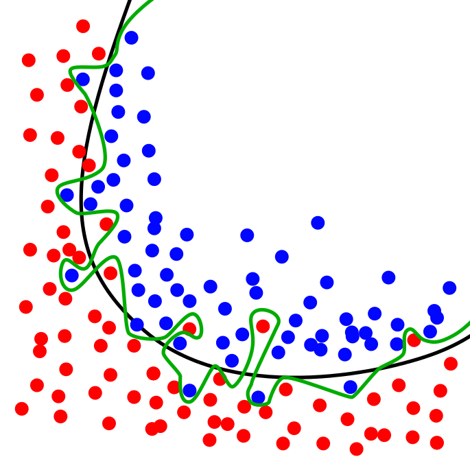
The worry there being that outside of the training data, it might not work as well for ‘real world’ data. For example the model represented by the green line in the image below (credit: Wikipedia), follows the sample data too closely and seems too good. On the other hand, the model represented by the black line, which is better.
Regularization helps with overfitting (artificially) penalizing the weights in the neural network. These weights are represented as peaks, and this reduces the peaks in the data. This ensure that the higher weights (peaks) don’t overshadow the rest of the data, and hence getting it to overfit. This diffusion of the weight vectors is sometimes also called weight decay.
Although there are a few regularization techniques for preventing overfitting (outlined below), these days in Deep Learning, L1 and L2 regression techniques are more favored over the others.
Cross validation: This is a method for finding the best hyper parameters for a model. E.g. in a gradient descent, this would be to figure out the stopping criteria. There are various ways to do this such as the holdout method, k-fold cross validation, leave-out cross validation, etc.
Step-wise regression: This method essentially is a serial step-by-step regression where one reduces the weakest variable. Step-wise regression essentially does multiple regression a number of times, each time removing the weakest correlated variable. At the end you are left with the variables that explain the distribution best. The only requirements are that the data is normally distributed, and that there is no correlation between the independent variables.
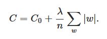
L1 regularization: In this method, we modify the cost function by adding the sum of the absolute values of the weights as the penalty (in the cost function). In L1 regularization the weights shrinks by a constant amount towards zero. L1 regularization is also called Lasso regression.
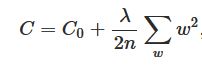
L2 regularization: In L2 regularization on the other hand, we re-scale the weight to a subset factor - it shrinks by an amount that is proportional to the weight (as outlined in the image below). This shrinking makes the weight smaller and is also sometimes called weight decay. To get this shrinking proportional, we take a squared mean of the weights , instead of the sum. At face value it might seem that the weight eventually get to zero, but that is not true; typically other terms cause the weights to increase. L2 regularization is also called Ridge regression.
Max-norm: This enforces a upper bound on the magnitude of the weight vector. The one area this helps is that a network cannot ’explode’ when the learning rates gets very high, as it is bounded. This is also called projected gradient descent.
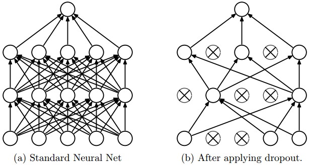
Dropout : Is very simple, and efficient and is used in conjunction with one of the previous techniques. Essentially it adds a probably on the neuron to keep it active, or ‘dropout’ by setting it to zero. Dropout doesn’t modify the cost function; it modifies the network itself as shown in the image below.
Increase training data: Whilst one can artificially expand the training set theoretically possible, in reality won’t work in most cases, especially in more complex networks. And in some cases one might think also to artificially expand the dataset, typically it is not cost effective to get a representative dataset.
Between L1 and L2 regularization, many say that L2 is preferred, but I think it depends on the problem statement. Say in a network, if a weight has a large magnitude, L2 regularization shrink the weight more than L1 and will better. Conversely, if the weight is small then L1 shrinks the weight more than L2 - and is better as it tends to concentrate the weight in fewer but more important connections in the network.
In closing, the key aspect to appreciate - the small weights (peaks) in a regularized network essentially means that as our input changes randomly (i.e. noise), it doesn’t have a huge impact to the network and its output. So this makes it difficult for the network to learn the noise and respond to that. Conversely, in an unregularized networks, that has higher weights (peaks), small random changes to those weights can have a larger impact to the behavior of the network and the information it carries.