Neural networks have a very interesting aspect – they can be viewed as a simple mathematical model that defines a function. For a given function $f(x)$ which can take any input value of $x$, there will be some kind a neural network satisfying that function. This hypothesis was proven almost 20 years ago (“ Approximation by Superpositions of a Sigmoidal Function ” and “ Multilayer feedforward networks are universal approximators ”) and forms the basis of much of #AI and #ML use cases possible .
It is this aspect of neural networks that allow us to map any process and generate a corresponding function. Unlike a function in Computer Science, this function isn’t deterministic; instead is confidence score of an approximation (i.e. a probability). The more layers in a neural network, the better this approximation will be.
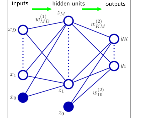
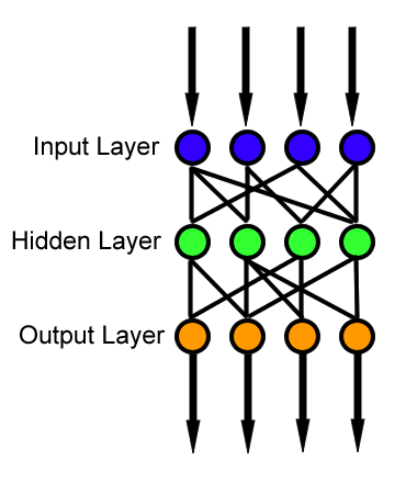
In a neural network, typically there is one input layer, one output layer, and one or more layers in the middle. To the external system, only the input layer (values of $x$), and the final output (output of the function $f(x)$) is visible, and the layers in the middle are not and are essentially hidden.
Each layer contains nodes, which are modeled after how the neurons in the brain works. The output of each node gets propagated along to the next layer. This output is the defining character of the node, and activates the node to pass on its value to the next node; this is very similar to how a neuron in the brain fires and works passing on the signal to the next neuron.
To make this generalization of function $f(x)$ outlined above to hold, that function needs to be a continuous function . A continuous function is one where small changes to the input value $x$, create small changes to the output of $f(x)$. If these outputs, are not small and the value jumps a lot then it is not continuous and it is difficult for the function to achieve the approximation required for them to be used in a neural network.
For a neural network to ‘learn’ – the network essentially has to use different weights and biases that has a corresponding change to the output, and possibly closer to the result we desire. Ideally, small changes to these weights and biases correspond to small changes in the output of the function. But one isn’t sure, until we train and test the result, to see that small changes don’t have bigger shifts that drastically move away from the desired result. It isn’t uncommon to see that one aspect of the result has improved, but others have not and overall skew the results.
In simple terms, an activation function is a node that is attached to the output of a neural network and maps the resulting value between 0 and 1. It is also used to connect two neural networks.
An activation function can be linear, or non-linear. A linear isn’t effective as its range is infinite. A non-linear with a finite range is more useful as it can be mapped as a curve, and then changes on this curve can be used to calculate the difference in the curve between two points.
There are many times of activation functions, each either its strengths. In this post, we discuss the following six:
- Sigmoid
- Tanh
- ReLU
- Leaky ReLU
- ELU
- Maxout
1. Sigmoid function
A sigmoid function can map any of input values into a probability – i.e., a value between 0 and 1. A sigmoid function is typically shown using a sigma ($\sigma$). Some also call the ($\sigma$) a logistic function. For any given input value, $ x $ the official definition of the sigmoid function is as follows:
$$\sigma(x) \equiv \frac{1}{1+e^{-x}}$$
If our inputs are $x_1, x_2,\ldots$, and their corresponding weights are $w_1, w_2,\ldots$, and a bias b, then the previous sigmoid definition is updated as follows:
$$\frac{1}{1+\exp(-\sum_j w_j x_j-b)}$$
When plotted, the sigmoid function will look plotted looks like this curve below. When we use this, in a neural network, we essentially end up with a smoothed-out function, unlike a binary function (also called a step function) – that is either 0, or 1.
For a given function, $f(x)$, as $x \rightarrow \infty$, $f(x)$ tends towards 1. And, as as $x \rightarrow -\infty$, $f(x)$ tends towards 0.
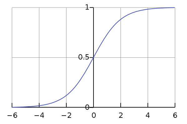
And this smoothness of $\sigma$ is what will create the small changes in the output that we desire - where small changes to the weights ($\Delta w_j$), and small changes to the bias ($\Delta b$) will produce small changes to the output ($\Delta output$).
Fundamentally, changing these weights and biases, is what can give us either a step function or small changes. We can show this as follows:
$$\Delta output \approx \sum_j (\frac{\partial \, output}{\partial w_j} \Delta w_j + \frac{\partial \, output}{\partial b} \Delta b)$$
One thing to be aware of is that the sigmoid function suffers from the vanishing gradient problem – the convergence between the various layers is very slow after a certain point – the neurons in previous layers don’t learn fast enough and are much slower than the neurons in later layers. Because of this, generally, a sigmoid is avoided.
2. Tanh (hyperbolic tangent function)
Tanh, is a variant of the sigmoid function, but still quite similar – it is a rescaled version and ranges from –1 to 1, instead of 0 and 1. As a result, its optimization is easier and is preferred over the sigmoid function. The formula for tanh is:
$$\tanh(x) \equiv \frac{e^x-e^{-z}}{e^X+e^{-x}}$$
Using, this we can show that:
$$\sigma(x) = \frac{1 + \tanh(x/2)}{2}$$.
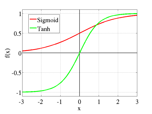
Tanh also suffers from the vanishing gradient problem. Both Tanh, and, Sigmoid are used in FNN (Feedforward neural network) – i.e. the information always moves forward and there isn’t any backprop.
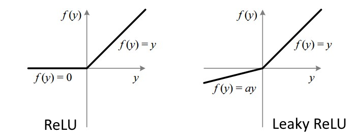
3. Rectified Linear Unit (ReLU)
A rectified linear unity ( ReLU ) is the most popular activation function that is used these days.
$$\sigma(x) = \begin{cases} x & x > 0\\ 0 & x \leq 0 \end{cases}$$
ReLU’s are quite popular for a couple of reasons – one, from a computational perspective, these are more efficient and simpler to execute - there isn’t any exponential operations to perform. And two, these don’t suffer from the vanishing gradient problem.
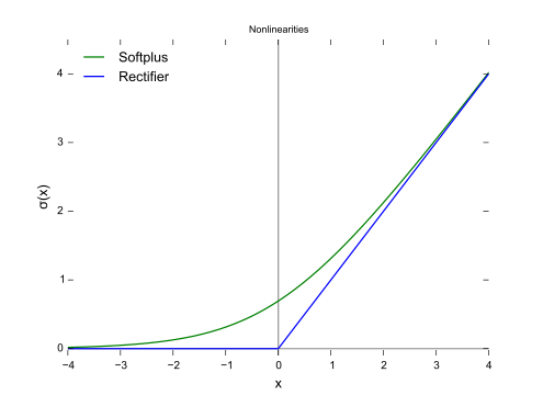
The one limitation ReLU’s have, is that their output isn’t in the probability space (i.e. can be >1), and can’t be used in the output layer.
As a result, when we use ReLU’s, we have to use a softmax function in the output layer. The output of a softmax function sums up to 1, and we can map the output as a probability distribution.
$$\sum_j a^L_j = \frac{\sum_j e^{z^L_j}}{\sum_k e^{z^L_k}} = 1.$$
Another issue that can affect ReLU’s is something called a dead neuron problem (also called a dying ReLU). This can happen when in the training dataset, some features have a negative value. When the ReLU is applied, those negative values become zero (as per the definition). If this happens at a large enough scale, the gradient will always be zero – and that node is never adjusted again (it is biased. and, weights never get changed) - essentially making it dead! The solution? Use a variation of the ReLU called a Leaky ReLU.
4. Leaky ReLU
A Leaky ReLU will usually allow a small slope $\alpha$ on the negative side; i.e that the value isn’t changed to zero, but rather something like 0.01. You can probably see the ‘leak’ in the image below. This ‘leak’ helps increase the range and we never get into the dying ReLU issue.
5. Exponential Linear Unit (ELU)
Sometimes a ReLU isn’t fast enough – over time, a ReLU’s mean output isn’t zero and this positive mean can add a bias for the next layer in the neural network; all this bias adds up and can slow the learning.
Exponential Linear Unit (ELU) can address this, by using an exponential function, which ensures that the mean activation is closer to zero. What this means, is that for a positive value, an ELU acts more like a ReLU and for the negative value it is bounded to -1 for $\alpha = 1$ – which puts the mean activation closer to zero.
$$\sigma(x) = \begin{cases} x & x \geqslant 0\\ \alpha (e^x - 1) & x < 0\end{cases}$$
When learning, this derivation of the slope is what is fed back (backprop) – so for this to be efficient, both the function and its derivative need to have a lower computation cost.

And finally, there is another variation that combines with ReLU and a Leaky ReLU called a Maxout function.
So, how do I pick one?
Choosing the ‘right’ activation function would of course depend on the data and problem at hand. My suggestion is to default to a ReLU as a starting step and remember ReLU’s are applied to hidden layers only. Use a simple dataset and see how that performs. If you see dead neurons than use a leaky ReLU or Maxout instead. It won’t make sense to use Sigmoid or Tanh these days for deep learning models but are useful for classifiers.
In summary, activation functions are a key aspect that fundamentally influences a neural network’s behavior and output. Having an appreciation and understanding of some of the functions is key to any successful ML implementation.